# -*- coding: utf-8 -*-
import numpy as np
import math
import matplotlib.pyplot as plt
import pandas as pd
import datetime
from scipy import interpolate
from pandas import DataFrame,Series

import numpy as np
import pywt

data = np.linspace(1, 4, 7)

# pywt.threshold方法讲解:
#               pywt.threshold(data,value,mode ='soft',substitute = 0 )
#               data:数据集,value:阈值,mode:比较模式默认soft,substitute:替代值,默认0,float类型

#data:   [ 1.   1.5  2.   2.5  3.   3.5  4. ]
#output:[ 6.   6.   0.   0.5  1.   1.5  2. ]
#soft 因为data中1小于2,所以使用6替换,因为data中第二个1.5小于2也被替换,2不小于2所以使用当前值减去2,,2.5大于2,所以2.5-2=0.5.....

print(pywt.threshold(data, 2, 'soft',6))


#data:   [ 1.   1.5  2.   2.5  3.   3.5  4. ]
#hard data中绝对值小于阈值2的替换为6,大于2的不替换
print (pywt.threshold(data, 2, 'hard',6))


#data:   [ 1.   1.5  2.   2.5  3.   3.5  4. ]
#data中数值小于阈值的替换为6,大于等于的不替换
print (pywt.threshold(data, 2, 'greater',6) )

print (data  )
#data:   [ 1.   1.5  2.   2.5  3.   3.5  4. ]
#data中数值大于阈值的,替换为6
print (pywt.threshold(data, 2, 'less',6) )
[6. 6. 0. 0.5 1. 1.5 2. ]
[6. 6. 2. 2.5 3. 3.5 4. ]
[6. 6. 2. 2.5 3. 3.5 4. ]
[1. 1.5 2. 2.5 3. 3.5 4. ]
[1. 1.5 2. 6. 6. 6. 6. ]
#!/usr/bin/env python
# -*- coding: utf-8 -*-

import numpy as np
import matplotlib.pyplot as plt

import pywt
import pywt.data


ecg = pywt.data.ecg()

data1 = np.concatenate((np.arange(1, 400),
                        np.arange(398, 600),
                        np.arange(601, 1024)))
x = np.linspace(0.082, 2.128, num=1024)[::-1]
data2 = np.sin(40 * np.log(x)) * np.sign((np.log(x)))

mode = pywt.Modes.smooth


def plot_signal_decomp(data, w, title):
    """Decompose and plot a signal S.
    S = An + Dn + Dn-1 + ... + D1
    """
    w = pywt.Wavelet(w)#选取小波函数
    a = data
    ca = []#近似分量
    cd = []#细节分量
    for i in range(5):
        (a, d) = pywt.dwt(a, w, mode)#进行5阶离散小波变换
        ca.append(a)
        cd.append(d)

    rec_a = []
    rec_d = []

    for i, coeff in enumerate(ca):
        coeff_list = [coeff, None] + [None] * i
        rec_a.append(pywt.waverec(coeff_list, w))#重构

    for i, coeff in enumerate(cd):
        coeff_list = [None, coeff] + [None] * i
        if i ==3:
            print(len(coeff))
            print(len(coeff_list))
        rec_d.append(pywt.waverec(coeff_list, w))

    fig = plt.figure()
    ax_main = fig.add_subplot(len(rec_a) + 1, 1, 1)
    ax_main.set_title(title)
    ax_main.plot(data)
    ax_main.set_xlim(0, len(data) - 1)

    for i, y in enumerate(rec_a):
        ax = fig.add_subplot(len(rec_a) + 1, 2, 3 + i * 2)
        ax.plot(y, 'r')
        ax.set_xlim(0, len(y) - 1)
        ax.set_ylabel("A%d" % (i + 1))

    for i, y in enumerate(rec_d):
        ax = fig.add_subplot(len(rec_d) + 1, 2, 4 + i * 2)
        ax.plot(y, 'g')
        ax.set_xlim(0, len(y) - 1)
        ax.set_ylabel("D%d" % (i + 1))


#plot_signal_decomp(data1, 'coif5', "DWT: Signal irregularity")
#plot_signal_decomp(data2, 'sym5',
#                   "DWT: Frequency and phase change - Symmlets5")
plot_signal_decomp(ecg, 'sym5', "DWT: Ecg sample - Symmlets5")


plt.show()
72
5

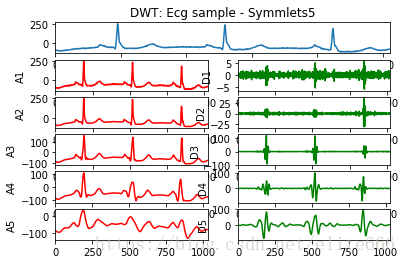
将数据序列进行小波分解,每一层分解的结果是上次分解得到的低频信号再分解成低频和高频两个部分。如此进过N层分解后源信号X被分解为:X = D1 + D2 + … + DN + AN 其中D1,D2,…,DN分别为第一层、第二层到等N层分解得到的高频信号,AN为第N层分解得到的低频信号。