如何用tf刚出一个高效的FM和DeepFM实操模型

前言

　　大名鼎鼎的FM模型，在工程界内是很受欢迎的，如何用tensorflow实现呢。

基础知识

线性LR模型：$y=w_0 + \sum_{i=1}^nw_i x_i$
FM：Factorization model，在线性模型LR的基础上，增加交叉组合特征，并用权重分解方法来解决稀疏特征的问题。

$y=w_0 + \sum_{i=1}^nw_i x_i + \sum_{i=1}^n \sum_{j=i+1}^nw_{i,j} x_i x_j$
稀疏特征下权重 $w_{i,j}$容易为零，不利于模型表达能力，采用权重矩阵分解方法 $[w_{i,j}]=[\left \langle v_i,v_j \right \rangle ]$，其中， $\left \langle v_i, v_j \right \rangle = \sum_k v_{i,k} v_{j,k}$。
$$\longrightarrow y=w_0 +\sum_{i=1}^nw_i x_i + \sum_{i=1}^n \sum_{j=i+1}^n\left \langle v_i, v_j \right \rangle x_i x_j$$
继续化简，如下：
$$\longrightarrow y=w_0 + \sum_{i=1}^n w_i x_i + \frac{1}{2}\sum_k [(\sum_{i=1}^n v_{i,k} x_j)^2-\sum_{i=1}^nv_{i,k}^2 x_j^2]$$
$\frac{\partial y}{\partial \theta}$梯度如下：
$$\frac{\partial y}{\partial \theta} = \left\{\begin{matrix} 1 & if \theta is w_0 \\ x_i & if \theta is w_i \\ [x_i \sum_{i=1}^n v_{i,k}x_i]-v_{i,k}x_i^2 & if \theta is v_{i,k} \end{matrix}\right.$$
也有人将最后项写作 $= x_i\sum_{j\neq i}v_{j,k}x_j$，等式变化下即可。
注：详细了解FTRL优化数学原理，请移步之前的博文 FTRL系列，绝对满足对原理及优化的深入解释。

用tf实现FM

　　因为tf会自动推导函数梯度，所以可以大大降低我们的计算难度。
　　剩下的主要问题就成了：
　　1） 输入特征是变长的。
　　2） 输入特征的值要参与计算。（这是由于业务需要）
　　关于输入，计划使用dataset来处理，因为方便好使。要解决变长特征的问题，通过下面的方法，关键脑回路要大一点。
　　变长特征在tf1.4的dataset里是不支持的，但对定长的输入是非常友好的；想办法绕过变长的限制，数据以\t分隔为三段，在dataset的基本处理之后使用tf.string_split切分，构造SparseTensor从而实现变长的批处理，并取出对应的特征值。这样，就可以既借助了dataset的方便之处，又可以实现变长特征的处理。
train-data example：

1^Iclick,show,title_kws^A李志林,title_kws^A股灾,title_kws^A演变,^I20.0,120.0,1,1,1$

import module tf1.4

import tensorflow as tf
from tensorflow.contrib.lookup import HashTable 
from tensorflow.contrib.lookup import TextFileIdTableInitializer 
from tensorflow.contrib.lookup import IdTableWithHashBuckets

dataset-input

## one-hot编码所用的vocab ##
vocab_file = './vocabulary.fm'
table_init = TextFileIdTableInitializer(vocab_file)
hash_table = HashTable(table_init, default_value=-1)
table_used = IdTableWithHashBuckets(hash_table, num_oov_buckets=10)
## feature parse ##
def input_fn(file_list, epoches=1, batch_size=1, shuffle=False):
  def parse_split(line):
    parse_res = tf.string_split([line], delimiter='\t')
    parse_res = parse_res.values
    labels    = tf.reshape(parse_res[0], [-1])
    labels    = tf.string_to_number(labels, out_type=tf.int32)
    return parse_res[1], parse_res[2], labels
  def parse_feature(k, v): ## 解析feature-value ##
    keys, values = [], []
    for i in range(batch_size):
      keys.append(tf.string_split([k[i]], ',').values)
      values.append(tf.string_to_number(tf.string_split([v[i]], ',').values, tf.float32))
    return keys, values
  def SparseTensorFeature(k, v): ## 提供list的训练样本 ##
    res = []
    for i in range(batch_size):
      keys, values   = k[i], v[i]
      feature_id     = table_used.lookup(keys)
      feature_id     = tf.expand_dims(feature_id, 1)
      sparse_example = tf.SparseTensor(indices=feature_id, values=values, dense_shape=(dense_len,))
      ## 通过feature查找ID-one-hot编码，构造SparseTensor ##
      res.append(sparse_example)
    return res
  def SparseTensorFeature_batch(k, v): ## 提供batch的训练样本 ##
    res = []
    for i in range(batch_size):
      keys, values   = k[i], v[i]
      feature_id     = table_used.lookup(keys)
      feature_id     = tf.expand_dims(feature_id, 1)
      sparse_example = tf.SparseTensor(indices=feature_id, values=values, dense_shape=(dense_len, ))
      sparse_example = tf.sparse_reshape(sp_input=sparse_example, shape=(1, dense_len))
      res.append(sparse_example)
    merge = tf.sparse_concat(axis=0, sp_inputs=res)
    return merge ## 这里的sparseTensor可以直接用来作sparse计算 ##

  dataset = tf.data.TextLineDataset(file_list)
  dataset = dataset.map(parse_split, num_parallel_calls=10)
  if shuffle: dataset = dataset.shuffle(buffer_size=5000)
  dataset = dataset.repeat(count = epoches)
  dataset = dataset.apply(tf.contrib.data.batch_and_drop_remainder(batch_size))
  dataset = dataset.make_one_shot_iterator()
  k, v, y = dataset.get_next()
  ## 将label \t feat1,feat2 \t value1,value2 这样用split('\t')来切分是长度固定的，就保证了所有的dataset附属函数都可用 ##
  keys, values         = parse_feature(k, v)
  #batch_sparse_feature = SparseTensorFeature(keys, values)
  batch_sparse_feature = SparseTensorFeature_batch(keys, values)
  ## 看你用哪种形式的输入[]还是batch形式的 ##
  return batch_sparse_feature, y

net-graph

  with tf.variable_scope('linear-part', reuse= tf.AUTO_REUSE):
    w = tf.get_variable(name= 'w', initializer = tf.random_normal((column_num, 1), mean= 0.0, stddev= 0.04), dtype= tf.float32, regularizer= regularizer)
    b = tf.get_variable(name= 'b', initializer = tf.zeros((1,1), dtype= tf.float32))
    y_linear = tf.matmul(x, w) + b # [batch_size, 1]
  with tf.variable_scope('non-linear-part', reuse= tf.AUTO_REUSE):
    Inner_dim = 8 
    W = tf.get_variable(name= 'W', initializer = tf.random_normal((column_num, Inner_dim), mean= 0.0, stddev= 0.04), dtype= tf.float32, regularizer= regularizer)
    y_non_linear = compute_cross(x, W)
  with tf.variable_scope('output-part', reuse= tf.AUTO_REUSE):
    output = tf.nn.sigmoid(tf.add(y_linear, y_non_linear))

batch-compute-node

def compute_cross(x, W): 
  # x batch SparseTensor #
  # sum_by_dim after [sum_by_batch(v_i x_i)]^2 - [sum_by_batch(v_i^2 x_i^2)]
  x_square = tf.square(x)
  W_square = tf.square(W)
  res1 = tf.square(tf.sparse_tensor_dense_matmul(x, W)) 
  res2 = tf.sparse_tensor_dense_matmul(x_square, W_square)
  res  = tf.reduce_sum(res1 - res2, axis=1, keep_dims=True)
  res  = tf.multiply(0.5, res)
  return res 

def compute_linear(x, w, b): 
  # x batch SparseTensor #
  res = tf.sparse_tensor_dense_matmul(x, w) + b 
  return res 

list-compute-node

def compute_cross_single(x, w): 
  y2= tf.multiply(tf.expand_dims(x, 2), w)
  y3= tf.square(tf.reduce_sum(y2, 1)) 
  y4= tf.reduce_sum(tf.square(y2), 1)
  y5= tf.multiply(0.5, tf.reduce_sum(y3 - y4, axis=1, keep_dims=True))
  return y5

def compute_cross(x, w): 
  res = []
  for i in range(batch_size):
    cur_example = x[i]
    cur_indices = cur_example.indices
    cur_values  = cur_example.values
    cur_weight  = tf.gather_nd(w, cur_indices) ## 用tf.gather_nd实现 tf.nn.embedding_lookup_sparse的效果 ##
    res.append(compute_cross_single(tf.expand_dims(cur_values, 0), cur_weight))
  return tf.squeeze(res, 2)
def compute_linear(x, w, b): 
  res = []
  for i in range(batch_size):
    cur_example = x[i]
    cur_indices = cur_example.indices
    cur_values  = cur_example.values
    cur_weight  = tf.gather_nd(w, cur_indices)
    res.append(tf.matmul(tf.expand_dims(cur_values, 0), cur_weight)+b)
  return tf.squeeze(res, 2)

notice

tensorflow里面的矩阵乘积计算

# 1) tf.matmul(dense_a, dense_b, a_is_sparse=False, b_is_sparse=False)
# 2) tf.sparse_matmul(dense_a, dense_b)
# 3) tf.sparse_tensor_dense_matmul(sparse_a, dense_b, a_is_sparse=False, b_is_sparse)
## 1/2 都是针对dense-matrix Tensor的计算，不过在指定矩阵是稀疏的时，会做计算优化 ##
## 3 才是对SparseTensor的计算，但是对b要求是dense的才可以。

关于tf.nn.embedding_lookup_sparse

扫描二维码关注公众号，回复： 2851337 查看本文章

## tf.nn.embedding_lookup_sparse 应该是最方便的稀疏计算方式
## tf.nn.embedding_lookup ## 是查找权重的便捷方法 ##

后续补充下使用embedding_lookup做DeepFM

用tf实现DeepFM

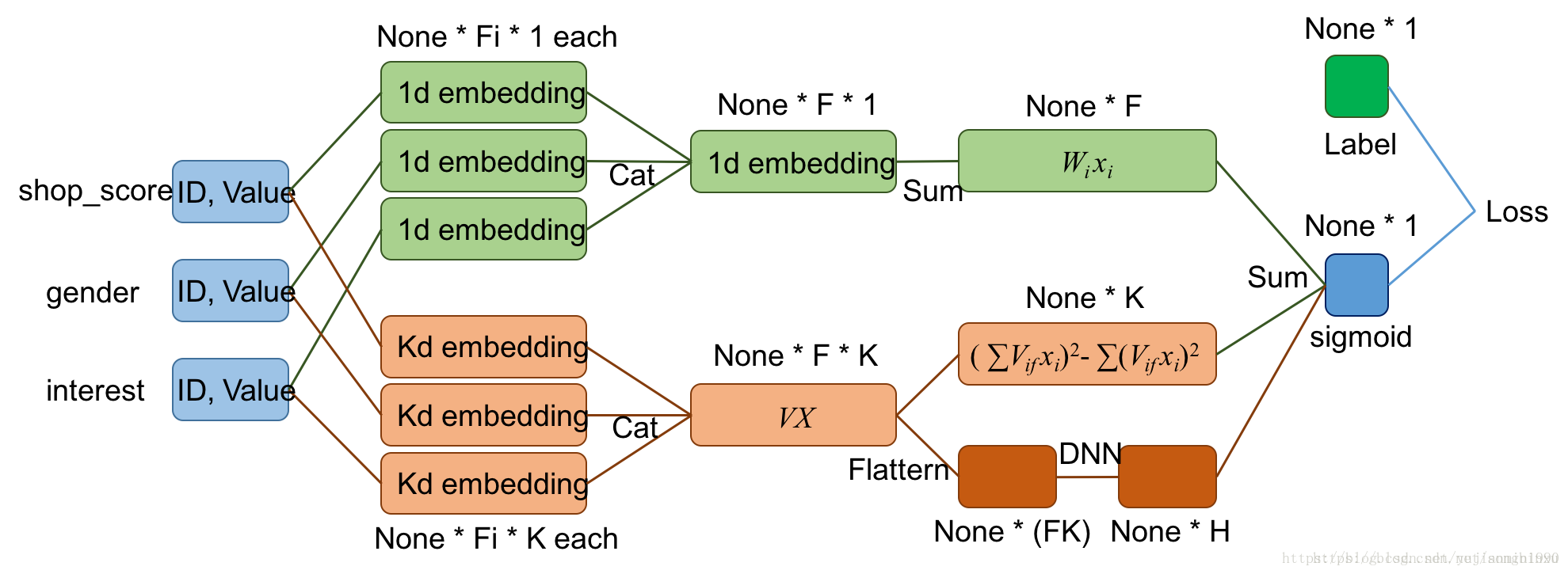
　　如果只是单纯的DeepFM的demo，很好实现，主要是应用场景下的各种歪要求和简洁考虑，就搞得好蛋疼的样子。DeepFM是在FM的基础上，共享输入给并行DNN网络，最后合并输出，下面给出DeepFM的一个比较清晰的计算流程图。

　　场景：变长特征。
　　矛盾：DeepFM在DNN的输入需要固定长度，就需要固定特征域的数量，每个域都映射成k-dim embedding，然后合并成固定尺寸的输入。
　　 解决一：好多DeepFM实现都是补全/删除特征，人为构造定长特征。
　　其缺点：是增加了DNN的学习难度，因为有些子特征是描述同一母特征的，人为被拆分导致不同位置上变稀疏且每个位置都需要学习权重。举个例子，假设title字段有好多个值，本来不同title_word就有好多词，都是为title_word这个字段特征贡献力量的。
　　 解决二：将母特征作为特征域，这样母特征域的数量还固定的，只是其下的子特征是不定长的（认为母特征是更具有描述性的特征粒度）。我们指定字段集作为母特征，其下的变长可能值作multi-hot编码，描述母特征。
　　 解决三：在图像处理中，有很多办法将不定长输入压缩为固定尺寸的 方法。
　　（FM没有这样的问题，是因为不需要固定尺寸，只是累和就足矣）
我们先按照解决方法一：（方案二用tf写得很丑）
dataset-input的函数修改

  ## 使用下面的x.indices, x.values 处理函数 ##
  def ListTensorFeature(k, v): 
    res_indice = []
    res_values = []
    for i in range(batch_size):
      keys, values = k[i], v[i]
      feature_id   = table_used.lookup(keys)
      res_indice.append(feature_id)
      res_values.append(values)
    return res_indice, res_values

compute-node

def compute_linear(x_indice, x_values, w, b):
  # w.shape = [feat_num_all, 1] #  x_indice.shape = [batch, feat_num]
  batch_weight = tf.nn.embedding_lookup(w, x_indice) ## batch x feat_num x 1
  batch_weight = tf.reduce_sum(batch_weight, 2)
  res          = tf.multiply(batch_weight, x_values) ## batch x feat_num 
  res          = tf.reduce_sum(res, 1, keep_dims=True) ## (batch, 1)
  res          = res + b
  return res
def embedding_layer(x_indice, x_values, W):
  batch_weight = tf.nn.embedding_lookup(W, x_indice) ## batch x feat_num x k
  return tf.multiply(batch_weight, tf.expand_dims(x_values, 2)) ## batch x feat_num x k
def compute_cross(x):
  res1         = tf.square(tf.reduce_sum(x, 1)) ## batch x k
  res2         = tf.reduce_sum(tf.square(x), 1) ## batch x k
  return tf.multiply(0.5, tf.reduce_sum(res1 - res2, 1, keep_dims=True)) ## (batch, 1)
def deep_input_batch(x):
  #return tf.layers.flatten(x) # batch x feat_num*k ## DNN不接受None的input ##
  return tf.reshape(x, [batch_size, Feat_num*Inner_dim])

net-graph

## net-graph ##
column_num  = dense_len
regularizer = tf.contrib.layers.l2_regularizer(0.01)
with tf.variable_scope('linear-part', reuse = tf.AUTO_REUSE):
  w = tf.get_variable(name='w', initializer= tf.random_normal(shape=(column_num, 1), mean= 0.0, stddev= 0.04), regularizer= regularizer)
  b = tf.get_variable(name='b', initializer= tf.zeros(shape=(1,1)))
  y_linear = compute_linear(x_indice, x_values, w, b)
with tf.variable_scope('non-linear-part', reuse = tf.AUTO_REUSE):
  W = tf.get_variable(name= 'W', initializer= tf.random_normal((column_num, Inner_dim), mean= 0.0, stddev= 0.04), regularizer= regularizer)
  embed_layer  = embedding_layer(x_indice, x_values, W)
  y_non_linear = compute_cross(embed_layer)
with tf.variable_scope('dnn-part', reuse = tf.AUTO_REUSE):
  input_dnn= deep_input_batch(embed_layer)
  hidden_1 = tf.layers.dense(inputs = input_dnn, units = 200, activation=tf.nn.relu, use_bias=True, name='hidden_1')
  hidden_2 = tf.layers.dense(inputs = hidden_1 , units = 120, activation=tf.nn.relu, use_bias=True, name='hidden_2')
  y_dnn_out= tf.layers.dense(inputs = hidden_2 , units = 1  , activation=None, use_bias=True, name='dnn_out')
with tf.variable_scope('merge-part', reuse = tf.AUTO_REUSE):
  merge_out= y_linear + y_non_linear + y_dnn_out
  y_output = tf.sigmoid(merge_out)

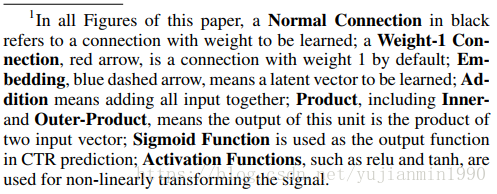
补充下DeepFM论文里面的结构图及对应连接线的解释

参考

1. Factorization Matchine
2. DeepFM
3. TFFM（tensorflow的FM分类接口） https://getstream.io/blog/factorization-recommendation-systems/