【tensorflow】保存模型、再次加载模型等操作

转自：https://blog.csdn.net/liuxiao214/article/details/79048136

由于经常要使用tensorflow进行网络训练，但是在用的时候每次都要把模型重新跑一遍，这样就比较麻烦；另外由于某些原因程序意外中断，也会导致训练结果拿不到，而保存中间训练过程的模型可以以便下次训练时继续使用。

所以练习了tensorflow的save model和load model。

参考于http://cv-tricks.com/tensorflow-tutorial/save-restore-tensorflow-models-quick-complete-tutorial/，这篇教程简单易懂！！

---

1、保存模型

# 首先定义saver类
saver = tf.train.Saver(max_to_keep=4)

# 定义会话
with tf.Session() as sess:

    sess.run(tf.global_variables_initializer())
    print "------------------------------------------------------"

    for epoch in range(300):
        if epoch % 10 == 0:
            print "------------------------------------------------------"
            # 保存模型
            saver.save(sess, "model/my-model", global_step=epoch)
            print "save the model"

        # 训练
        sess.run(train_step)
    print "------------------------------------------------------"

• 1
• 2
• 3
• 4
• 5
• 6
• 7
• 8
• 9
• 10
• 11
• 12
• 13
• 14
• 15
• 16
• 17
• 18
• 19

注意点：

1. 创建saver时，可以指定需要存储的tensor，如果没有指定，则全部保存。

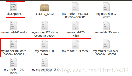
2. 创建saver时，可以指定保存的模型个数，利用max_to_keep=4，则最终会保存4个模型（下图中我保存了160、170、180、190step共4个模型）。

3. saver.save()函数里面可以设定global_step，说明是哪一步保存的模型。

4. 程序结束后，会生成四个文件：存储网络结构.meta、存储训练好的参数.data和.index、记录最新的模型checkpoint。

如：

2、加载模型

def load_model():
    with tf.Session() as sess:
        saver = tf.train.import_meta_graph('model/my-model-290.meta')
        saver.restore(sess, tf.train.latest_checkpoint("model/"))

• 1
• 2
• 3
• 4
• 5

注意点：

1. 首先import_meta_graph，这里填的名字meta文件的名字。然后restore时，是检查checkpoint，所以只填到checkpoint所在的路径下即可，不需要填checkpoint，不然会报错“ValueError: Can’t load save_path when it is None.”。

2. 后面根据具体例子，介绍如何利用加载后的模型得到训练的结果，并进行预测。

3、线性拟合例子

首先，上代码。

import tensorflow as tf
import numpy as np

def train_model():

    # prepare the data
    x_data = np.random.rand(100).astype(np.float32)
    print x_data
    y_data = x_data * 0.1 + 0.2
    print y_data

    # define the weights
    W = tf.Variable(tf.random_uniform([1], -20.0, 20.0), dtype=tf.float32, name='w')
    b = tf.Variable(tf.random_uniform([1], -10.0, 10.0), dtype=tf.float32, name='b')
    y = W * x_data + b

    # define the loss
    loss = tf.reduce_mean(tf.square(y - y_data))
    train_step = tf.train.GradientDescentOptimizer(0.5).minimize(loss)

    # save model
    saver = tf.train.Saver(max_to_keep=4)

    with tf.Session() as sess:

        sess.run(tf.global_variables_initializer())
        print "------------------------------------------------------"
        print "before the train, the W is %6f, the b is %6f" % (sess.run(W), sess.run(b))

        for epoch in range(300):
            if epoch % 10 == 0:
                print "------------------------------------------------------"
                print ("after epoch %d, the loss is %6f" % (epoch, sess.run(loss)))
                print ("the W is %f, the b is %f" % (sess.run(W), sess.run(b)))
                saver.save(sess, "model/my-model", global_step=epoch)
                print "save the model"
            sess.run(train_step)
        print "------------------------------------------------------"

def load_model():
    with tf.Session() as sess:
        saver = tf.train.import_meta_graph('model/my-model-290.meta')
        saver.restore(sess, tf.train.latest_checkpoint("model/"))
        print sess.run('w:0')
        print sess.run('b:0')

train_model()
load_model()

• 1
• 2
• 3
• 4
• 5
• 6
• 7
• 8
• 9
• 10
• 11
• 12
• 13
• 14
• 15
• 16
• 17
• 18
• 19
• 20
• 21
• 22
• 23
• 24
• 25
• 26
• 27
• 28
• 29
• 30
• 31
• 32
• 33
• 34
• 35
• 36
• 37
• 38
• 39
• 40
• 41
• 42
• 43
• 44
• 45
• 46
• 47
• 48

1. 首先定义了y=ax+b的线性关系，a=0.1，b=0.2，然后给定训练数据集，w是-20.0到20.0之间的任意数，b是-10.0到10.0之间的任意数。

2. 然后定义损失函数，定义随机梯度下降训练器。

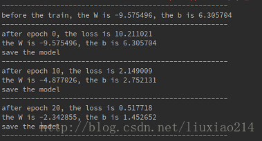
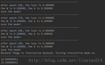
3. 定义saver后进入训练阶段，边训练边保存模型。并输出中间的训练loss，w和b。可以看到w和b在逐步接近我们设定的0.1和0.2。

4. 在load_model函数中，我们首先利用第2小节中的方法加载模型，然后就可以根据模型中权值的名字，打印其结果。

注意：

这里说明一点，如何知道tensor的名字，最好是定义tensor的时候就指定名字，如上面代码中的name='w'，如果你没有定义name，tensorflow也会设置name，只不过这个name就是根据你的tensor或者操作的性质，像上面的w，这是“Variable:0”，loss则是“Mean:0”。所以最好还是自己定义好name。

最后给出结果：

4、卷积神经网络例子

首先，上代码：

import tensorflow as tf
import numpy as np
import os

def load_data(resultpath):

    datapath = os.path.join(resultpath, "data10_4.npz")
    if os.path.exists(datapath):
        data = np.load(datapath)
        X, Y = data["X"], data["Y"]
    else:
        X = np.array(np.arange(30720)).reshape(10, 32, 32, 3)
        Y = [0, 0, 1, 1, 2, 2, 3, 3, 2, 0]
        X = X.astype('float32')
        Y = np.array(Y)
        np.savez(datapath, X=X, Y=Y)
        print('Saved dataset to dataset.npz.')
    print('X_shape:{}\nY_shape:{}'.format(X.shape, Y.shape))
    return X, Y

def define_model(x):

    x_image = tf.reshape(x, [-1, 32, 32, 3])
    print x_image.shape

    def weight_variable(shape):
        initial = tf.truncated_normal(shape, stddev=0.1)
        return tf.Variable(initial, name="w")

    def bias_variable(shape):
        initial = tf.constant(0.1, shape=shape)
        return tf.Variable(initial, name="b")

    def conv3d(x, W):
        return tf.nn.conv2d(x, W, strides=[1, 1, 1, 1], padding='SAME')

    def max_pool_2d(x):
        return tf.nn.max_pool(x, ksize=[1, 3, 3, 1], strides=[1, 3, 3, 1], padding='SAME')

    with tf.variable_scope("conv1"):  # [-1,32,32,3]
        weights = weight_variable([3, 3, 3, 32])
        biases = bias_variable([32])
        conv1 = tf.nn.relu(conv3d(x_image, weights) + biases)
        pool1 = max_pool_2d(conv1)  # [-1,11,11,32]

    with tf.variable_scope("conv2"):
        weights = weight_variable([3, 3, 32, 64])
        biases = bias_variable([64])
        conv2 = tf.nn.relu(conv3d(pool1, weights) + biases)
        pool2 = max_pool_2d(conv2) # [-1,4,4,64]

    with tf.variable_scope("fc1"):
        weights = weight_variable([4 * 4 * 64, 128]) # [-1,1024]
        biases = bias_variable([128])
        fc1_flat = tf.reshape(pool2, [-1, 4 * 4 * 64])
        fc1 = tf.nn.relu(tf.matmul(fc1_flat, weights) + biases)
        fc1_drop = tf.nn.dropout(fc1, 0.5) # [-1,128]

    with tf.variable_scope("fc2"):
        weights = weight_variable([128, 4])
        biases = bias_variable([4])
        fc2 = tf.matmul(fc1_drop, weights) + biases # [-1,4]

    return fc2

def train_model():

    x = tf.placeholder(tf.float32, shape=[None, 32, 32, 3], name="x")
    y_ = tf.placeholder('int64', shape=[None], name="y_")

    initial_learning_rate = 0.001
    y_fc2 = define_model(x)
    y_label = tf.one_hot(y_, 4, name="y_labels")

    loss_temp = tf.losses.softmax_cross_entropy(onehot_labels=y_label, logits=y_fc2)
    cross_entropy_loss = tf.reduce_mean(loss_temp)

    train_step = tf.train.AdamOptimizer(learning_rate=initial_learning_rate, beta1=0.9, beta2=0.999,
                                        epsilon=1e-08).minimize(cross_entropy_loss)

    correct_prediction = tf.equal(tf.argmax(y_fc2, 1), tf.argmax(y_label, 1))
    accuracy = tf.reduce_mean(tf.cast(correct_prediction, tf.float32))

    # save model
    saver = tf.train.Saver(max_to_keep=4)
    tf.add_to_collection("predict", y_fc2)

    with tf.Session() as sess:

        sess.run(tf.global_variables_initializer())
        print "------------------------------------------------------"
        X, Y = load_data("model1/")
        X = np.multiply(X, 1.0 / 255.0)
        for epoch in range(200):

            if epoch % 10 == 0:
                print "------------------------------------------------------"

                train_accuracy = accuracy.eval(feed_dict={x: X, y_: Y})
                train_loss = cross_entropy_loss.eval(feed_dict={x: X, y_: Y})

                print ("after epoch %d, the loss is %6f" % (epoch, train_loss))
                print ("after epoch %d, the acc is %6f" % (epoch, train_accuracy))

                saver.save(sess, "model1/my-model", global_step=epoch)
                print "save the model"

            train_step.run(feed_dict={x: X, y_: Y})

        print "------------------------------------------------------"

def load_model():

    # prepare the test data
    X = np.array(np.arange(6144, 12288)).reshape(2, 32, 32, 3)
    Y = [3, 1]
    Y = np.array(Y)
    X = X.astype('float32')
    X = np.multiply(X, 1.0 / 255.0)
    with tf.Session() as sess:

        # load the meta graph and weights
        saver = tf.train.import_meta_graph('model1/my-model-190.meta')
        saver.restore(sess, tf.train.latest_checkpoint("model1/"))

        # get weights
        graph = tf.get_default_graph()
        fc2_w = graph.get_tensor_by_name("fc2/w:0")
        fc2_b = graph.get_tensor_by_name("fc2/b:0")

        print "------------------------------------------------------"
        print sess.run(fc2_w)
        print "#######################################"
        print sess.run(fc2_b)
        print "------------------------------------------------------"

        input_x = graph.get_operation_by_name("x").outputs[0]

        feed_dict = {"x:0":X, "y_:0":Y}
        y = graph.get_tensor_by_name("y_labels:0")
        yy = sess.run(y, feed_dict)
        print yy
        print "the answer is: ", sess.run(tf.argmax(yy, 1))
        print "------------------------------------------------------"

        pred_y = tf.get_collection("predict")
        pred = sess.run(pred_y, feed_dict)[0]
        print pred, '\n'

        pred = sess.run(tf.argmax(pred, 1))
        print "the predict is: ", pred
        print "------------------------------------------------------"

        acc = graph.get_operation_by_name("acc")
        acc = sess.run(acc, feed_dict)
        print "the accuracy is: ", acc
        print "------------------------------------------------------"

#train_model()
load_model()

• 1
• 2
• 3
• 4
• 5
• 6
• 7
• 8
• 9
• 10
• 11
• 12
• 13
• 14
• 15
• 16
• 17
• 18
• 19
• 20
• 21
• 22
• 23
• 24
• 25
• 26
• 27
• 28
• 29
• 30
• 31
• 32
• 33
• 34
• 35
• 36
• 37
• 38
• 39
• 40
• 41
• 42
• 43
• 44
• 45
• 46
• 47
• 48
• 49
• 50
• 51
• 52
• 53
• 54
• 55
• 56
• 57
• 58
• 59
• 60
• 61
• 62
• 63
• 64
• 65
• 66
• 67
• 68
• 69
• 70
• 71
• 72
• 73
• 74
• 75
• 76
• 77
• 78
• 79
• 80
• 81
• 82
• 83
• 84
• 85
• 86
• 87
• 88
• 89
• 90
• 91
• 92
• 93
• 94
• 95
• 96
• 97
• 98
• 99
• 100
• 101
• 102
• 103
• 104
• 105
• 106
• 107
• 108
• 109
• 110
• 111
• 112
• 113
• 114
• 115
• 116
• 117
• 118
• 119
• 120
• 121
• 122
• 123
• 124
• 125
• 126
• 127
• 128
• 129
• 130
• 131
• 132
• 133
• 134
• 135
• 136
• 137
• 138
• 139
• 140
• 141
• 142
• 143
• 144
• 145
• 146
• 147
• 148
• 149
• 150
• 151
• 152
• 153
• 154
• 155
• 156
• 157
• 158
• 159
• 160

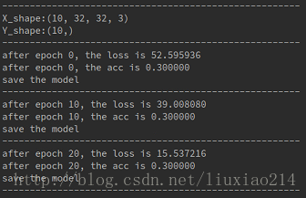
1. 定义了一个简单的卷积神经网络：有两个卷积层、两个池化层和两个全连接层。

2. 加载的数据是无意义的数据，模拟的是10张32x32的RGB图像，共4个类别0、1、2、3。

3. 在train_model中，定义了一下可能需要的tensor或操作的name，以便加载模型后使用。

4. 在定义saver时，对要预测的值fc2添加了进去，并定义name为“predict”，以便在预测时使用。

5. 在load_model中，输出了一些中间结果，如最后一层的W和b的值。然后根据随机创建的测试数据集，模拟2张32x32的RGB图，预测这两张图像的类别，放入feed_dict，输出预测结果。

6. 首先返回了测试数据的真实标签。

7. 返回的是一个2位矩阵，第一行是第一个图像的结果，长度为4，因为有4个种类，第二行是第二张图像的结果。所以我们要将这个返回我们熟悉的0、1、2、3，只要返回最大值的下标即可。使用tf.argmax即可。

8. 返回准确度，不知道为什么，是None，后面再找找问题出在哪。

给出输出结果：

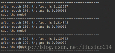
虽然我们的训练数据和测试数据都是随机无意义的数，所以这个预测结果也不必认真纠结。

5、fine-tuning

使用已经预训练好的模型，自己fine-tuning。

1、首先获得pre-traing的graph结构，saver = tf.train.import_meta_graph('my_test_model-1000.meta')

2、加载参数，saver.restore(sess,tf.train.latest_checkpoint('./'))

3、准备feed_dict，新的训练数据或者测试数据。这样就可以使用同样的模型，训练或者测试不同的数据。

4、如果想在已有的网络结构上添加新的层，如前面卷积网络，获得fc2时，然后添加了一个全连接层和输出层。

pred_y = graph.get_tensor_by_name("fc2/add:0")

        ## add the new layers
        weights = tf.Variable(tf.truncated_normal([4, 6], stddev=0.1), name="w")
        biases = tf.Variable(tf.constant(0.1, shape=[6]), name="b")
        conv1 = tf.matmul(pred_y, weights) + biases
        output1 = tf.nn.softmax(conv1)

• 1
• 2
• 3
• 4
• 5
• 6
• 7

5、只要加载模型的前一部分，然后从后面开始fine-tuning。

# pre-train and fine-tuning
        fc2 = graph.get_tensor_by_name("fc2/add:0")
        fc2 = tf.stop_gradient(fc2)  # stop the gradient compute
        fc2_shape = fc2.get_shape().as_list()

        # fine -tuning
        new_nums = 6
        weights = tf.Variable(tf.truncated_normal([fc2_shape[1], new_nums], stddev=0.1), name="w")
        biases = tf.Variable(tf.constant(0.1, shape=[new_nums]), name="b")
        conv2 = tf.matmul(fc2, weights) + biases
        output2 = tf.nn.softmax(conv2)

• 1
• 2
• 3
• 4
• 5
• 6
• 7
• 8
• 9
• 10
• 11

7、知识点

1、.meta文件：一个协议缓冲，保存tensorflow中完整的graph、variables、operation、collection。

2、checkpoint文件：一个二进制文件，包含了weights, biases, gradients和其他variables的值。但是0.11版本后的都修改了，用.data和.index保存值，用checkpoint记录最新的记录。

3、在进行保存时，因为meta中保存的模型的graph，这个是一样的，只需保存一次就可以，所以可以设置saver.save(sess, 'my-model', write_meta_graph=False)即可。

4、如果想设置每多长时间保存一次，可以设置saver = tf.train.Saver(keep_checkpoint_every_n_hours=2)，这个是每2个小时保存一次。

5、如果不想保存所有变量，可以在创建saver实例时，指定保存的变量，可以以list或者dict的类型保存。如：

w1 = tf.Variable(tf.random_normal(shape=[2]), name='w1')
w2 = tf.Variable(tf.random_normal(shape=[5]), name='w2')
saver = tf.train.Saver([w1,w2])