使用LSTM预测股价，特征：19个指标5天历史数据

LSTM介绍

LSTM是具有时间特性的神经网络，我们利用LSTM预测时间序列——股价。 
从文本到股价，LSTM的输入特征和网络结构都有哪些变化呢？ 
我们先看一个简单的RNN结构。与普通的全连接层神经网络的权重更新沿着一层层隐藏层网络不同，RNN的权重更新有两个方向，一个是像传统神经网络沿着输入层隐藏层更新，即图中的U和V的权重矩阵，一个是沿着St-2,St-1,St,St+1...的状态层更新，即途中的W权重矩阵。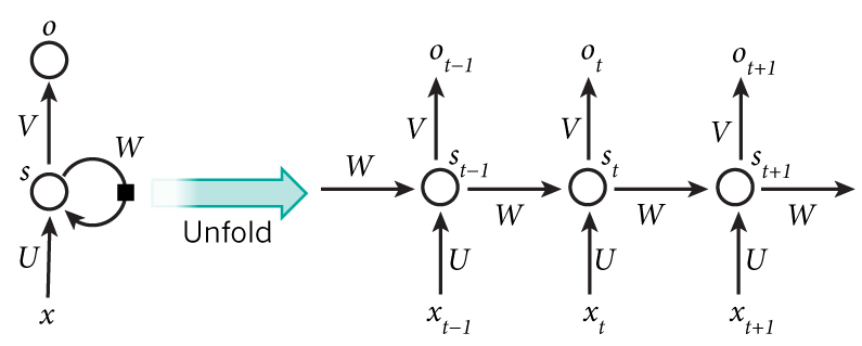 
 
对于传统的神经网络，假如输入数据的格式是[100,5]，即100个样本，特征是5，那么输入神经元的个数是[5] 
对于RNN处理的时间序列，应该是什么样的呢？ 
首先我们知道RNN可以处理文本信息。例如，这句话。

我昨天上学迟到了

利用python的jieba分词

1. jieba.cut('我昨天上学迟到了')

得到这样的句式结构。

我 昨天 上学 迟到 了

那么实际上输入输出是这样的：

输入	标签
s	我
我	昨天
昨天	上学
上学	迟到
迟到	了

或者

input: [“Jack”, “and”, “Jill”, “went”], label: [“up”]

input: [“and”, “Jill”, “went”, “up”], label: [“the”]

input: [“Jill”, “went”, “up”, “the”], label: [“hill”]

input: [“went”, “up”, “the”, “hill”], label: [“.”]

做向量化和one-hot编码得到，这里的one-hot不是真正的编码，是我举例的，真正的维度要高得多，这里假设是10维

输入	标签
0000000001	0000000010
0000000010	0000000100
0000000100	0000001000
0000001000	0000010000
0000010000	0000100000

输入数据的格式（100，20，10） 
100是序列个数，一篇文章句子的个数。 
20是时间步，就是句子最大能容纳的词数，词数少的句子补齐。 
10是每个时间步的维度，就是词向量维度。

开始建模

数据：香港恒生指数 
指标：'Closing Price', 'Open Price', 'High price', 'Low Price','Volume','MACD', 'CCI', 'ATR', 'BOLL_MID', 'EMA20','MA10','MTM6', 'MA5','MTM12', 'ROC', 'SMI', 'WVAD', 'US Dollar Index','HIBOR' 
日期：2008-07-02' 至 '2016-09-30'

首先，定义一个求t-5,t-4,t-3,t-2,t-1时刻的特征指标的函数，也就是之前的19维特征，现在变成了19*（5+1）=114维的特征。+1是因为考虑t时刻本身的特征。

1. def series_to_supervised(data, n_in=1, n_out=1, dropnan=True):
2. #if n_in=2, t-2,t-1,t
3. n_vars = 1 if type(data) is list else data.shape[1] #return feature numbers
4. df = DataFrame(data)
5. cols, names = list(), list()
6. # input sequence (t-n_in, ... t-1)
7. for i in range(n_in, 0, -1):#print n_int to i in inverted order[n_in,n_in-1,...,1]
8. cols.append(df.shift(i))
9. names += [('var%d(t-%d)' % (j+1, i)) for j in range(n_vars)]
10. # forecast sequence (t, t+1, ... t+n)
11. for i in range(0, n_out):
12. cols.append(df.shift(-i))
13. if i == 0:
14. names += [('var%d(t)' % (j+1)) for j in range(n_vars)]
15. else:
16. names += [('var%d(t+%d)' % (j+1, i)) for j in range(n_vars)]
17. # put it all together
18. agg = concat(cols, axis=1)
19. agg.columns = names
20. # drop rows with NaN values
21. if dropnan:
22. agg.dropna(inplace=True)
23. return agg

看一下用这个函数处理完后dataset的格式，主要是columns的feature列有变化。处理完后的变量叫reframed，会在后面的代码里看到它的具体来源。 
这里var1..var19就是那19个特征指标。

1. In [42]:reframed.columns
2. Out[42]:
3. Index(['var1(t-5)', 'var2(t-5)', 'var3(t-5)', 'var4(t-5)', 'var5(t-5)',
4. 'var6(t-5)', 'var7(t-5)', 'var8(t-5)', 'var9(t-5)', 'var10(t-5)',
5. ...
6. 'var10(t)', 'var11(t)', 'var12(t)', 'var13(t)', 'var14(t)', 'var15(t)',
7. 'var16(t)', 'var17(t)', 'var18(t)', 'var19(t)'],
8. dtype='object', length=114)

首先导入数据，去掉多余的Time列

1. from pandas import read_excel,DataFrame,concat
2. from matplotlib import plt
3. import matplotlib.finance as mpf
4. import numpy as np
5. import pandas as pd
6. import matplotlib.plot as plt
7. # load dataset
8. dataset = read_excel('RawData.xlsx', header=0, index_col=0)
9. dataset=dataset.drop('Time',1)

对数据进行预处理，包括encoder,归一化,人为的特征选择。

1. #transfer dataframe to arrays
2. values = dataset.values
3. # integer encode direction
4. # 选出label列做encoder，也可以尝试hot encoder
5. encoder = LabelEncoder()
6. values[:,4] = encoder.fit_transform(values[:,4])
7. # ensure all data is float
8. values = values.astype('float32')
9. # normalize features
10. scaler = MinMaxScaler(feature_range=(0, 1))
11. #label encode 的整数也要被归一化到0,1间
12. scaled = scaler.fit_transform(values)
13. # frame as supervised learning
14. reframed = series_to_supervised(scaled, 5, 1)
15. # drop columns we don't want to use　to predict
16. # 去掉不需要的特征
17. #reframed.drop(reframed.columns[[9,10,11,12,13,14,15]], axis=1, inplace=True)
18. print(reframed.head())

划分训练集和测试集，这里需要注意不要shuffle打乱样本顺序。 
我们选择reframed的0~95（不包含96）作为特征，96是t天的closing price，作为label，97~113是t天剩下的指标，所以不选，在做股价预测切忌把t天的时间信息参杂进去。

1. # split into train and test sets
2. values = reframed.values
3. n_train_hours = 365 * 2
4. # 选取所有指标的t-5到t-1作为feature,closing Price的t时刻作为label
5. train = values[:n_train_hours, :96]
6. test = values[n_train_hours:, :96]
7. # split into input and outputs
8. # 将close_price作为y,Closing Price是第0个特征，也就是reframed的第95个特征
9. train_X, train_y = train[:, 0:-1], train[:, -1]
10. test_X, test_y = test[:, 0:-1], test[:, -1]
11. # reshape input to be 3D [samples, timesteps, features]
12. # 将每一行切割开，每一行作为一个输入样本，所以每个样本有时间上的延迟关联性。
13. train_X = train_X.reshape((train_X.shape[0], 1, train_X.shape[1]))
14. test_X = test_X.reshape((test_X.shape[0], 1, test_X.shape[1]))
15. print(train_X.shape, train_y.shape, test_X.shape, test_y.shape)

接下来利用基于tensorflow的keras搭建一个简易的LSTM网络。 
注意输入张量的格式，是[1,95]，1是步长，就是每次我们的rolling window移动1个时间单位，因为我们是从第6天开始用前5天的数据，预测第7天的股价。也就是t天预测t+1天，所以步长是1。

1. # design network
2. from keras.models import Sequential
3. from keras.layers import Dense, Activation, LSTM
5. model = Sequential()
6. model.add(LSTM(50, input_shape=(train_X.shape[1],train_X.shape[2])))
7. model.add(Dense(1))
8. model.compile(loss='mae', optimizer='adam')
9. # fit network
10. history = model.fit(train_X, train_y, epochs=40, batch_size=72, validation_data=(test_X, test_y), verbose=2, shuffle=False)
11. # plot history
12. plt.plot(history.history['loss'], label='train')
13. plt.plot(history.history['val_loss'], label='test')
14. plt.legend()
15. plt.show()
16. test_predict=model.predict(test_X)

评估

预测得到的test_predict就是基于测试集的数据预测的股价，可以和真实的股价test_y做一下对比。

1. dataset.index=pd.to_datetime(dataset.index,format='%Y%m%d')
2. test_df=pd.DataFrame({'predict':test_predict.reshape(test_predict.shape[0]),'real':test_y},index=dataset.index[n_train_hours+5:])
3. #test_df['predict'].plot(label='predict')
4. #test_df['real'].plot(label='real')
5. #plt.legend()
6. #plt.title('Closing Price')
8. #Undo the scaling
9. #去归一化，得到预测股价和真实股价，之前用train直接做的归一化scaler必须要19个特征的维度，这里重新用单个特征（收盘价）做归一化和去归一化
10. scaler_ClosingPrice = MinMaxScaler(feature_range=(0, 1))
11. ClosingPrice_scaled=scaler_ClosingPrice.fit_transform(dataset['Closing Price'].values.astype('float32').reshape(-1,1))
12. predict_close=scaler_ClosingPrice.inverse_transform(test_df['predict'].values.astype('float32').reshape(-1,1))
13. real_close=scaler_ClosingPrice.inverse_transform(test_df['real'].values.astype('float32').reshape(-1,1))
15. #画出股价图
16. test_df=pd.DataFrame({'predict':predict_close.reshape(predict_close.shape[0]),'real':real_close.reshape(real_close.shape[0])},index=dataset.index[n_train_hours+5:])
17. test_df['predict'].plot(label='predict')
18. test_df['real'].plot(label='real')
19. plt.legend()
20. plt.title('Closing Price')

这里乍一看似乎是拟合的不错，但仔细看可以看出，预测股价相对于真实股价有一些的滞后性，所以我们试着比较一下模型趋势预测的准确性。

定义一个在当天判断num天后股价是否会上涨的函数，返回一个bool类型的趋势数据

1. def price_is_rise(X,num=1):
2. close_dif=[]
3. is_rise=[]
4. for i in range(0,len(X)-num):
5. close_dif.append(X[i+num]-X[i])
6. if close_dif[i]>0:
7. is_rise.append(True)
8. else:
9. is_rise.append(False) #Get price rising flag on next day
10. return is_rise
12. predict_is_rise=price_is_rise(test_df['predict'],1)
13. real_is_rise=price_is_rise(test_df['real'],1)

定义一个判断两个趋势数据相等准确率的函数

1. def trend_accuracy(data1,data2):
2. correct_score=0
3. inequalerror='Data1 and data2 should has same length.'
4. if len(data1)!=len(data2):
5. raise inequalerror
6. for i in range(0,len(data1)):
7. if predict_is_rise[i]==real_is_rise[i]:
8. correct_score+=1
10. return correct_score/len(data1)
12. trend_accuracy(predict_is_rise,real_is_rise)

我的模型得到的趋势准确率：

1. Out[35]: 0.48962336664104533

看来不高，和人为猜测差不多，当然，还需要不断完善特征和模型的参数。 
比如特征，不能单纯的用量、价的值，要用差值。比如输入数据，要经过滤波处理。 

实际上，就算准确率高也是过拟合，这种模型基本没什么意义。如果任何一种模型的预测准确率能远高于50%，那将存在很恐怖的超额收益，这部分收益会迅速被市场吞噬掉，那么早就会有人赚到钱了，市场有效性假说不再成立。