A cylindrical scanning setup with an optical distance probe is non-contact, universal and fast. With a probe with 5 mm range, circular tracks on freeform surfaces can be measured rapidly with minimized system dynamics. By applying a metrology frame relative to which the position of the probe and the product are measured, most stage errors are eliminated from the metrology loop. Because the probe is oriented perpendicular to the aspherical best-fit of the surface, the sensitivity to tangential errors is reduced. This allows for the metrology system to be 2D. The machine design consists of the motion system, the metrology system and the non-contact probe.
2.1 Conceptual considerations
Based on the review of existing measurement methods, some fundamental choices can be made with regard to the characteristics of the measurement method.
Method
Although imaging techniques such as phase-shifting interferometry provide accurate, non-contact and very fast measurement, they are not universal and are difficult to scale to the required dimensions. Single point scanning methods are slower and the moving of components generally requires more effort to obtain high accuracy, but they are in principle capable of universal measurement in a large volume. With a suitable probe, fast non-contact measurement is possible.
Probe type
Several principles can be used for probing the surface, as summarized in (Schwenke et al., 2002; Weckenmann et al., 2006). Optical probes are truly non-contact and especially single point sensors allow for scanning speeds in the order of meters per second. Care must be taken when applying an optical technique, since measurement relies on reflection of the surface under test, which generally is sensitive to imperfections such as dust and scratches.
Semi-contact scanning probe microscopy principles, such as Atomic Force Probes, can be used to measure the distance to a surface by keeping the stylus at constant distance or using it tapping mode. Since the tip is extremely fragile, scanning speeds are much smaller than one millimeter per second, which is similar to contact probes. Capacitive probes are capable of high-accuracy, but can only be applied to metallic surfaces and are thus not suitable for transmission optics. The same goes for other non-contact sensors such as Eddy-current sensors. Ultrasonic sensors have not been found to provide the required resolution.
Only optical probes are truly non-contact, have sufficient accuracy and allow for high scanning speeds. Hence, they are the probe type of choice. The global surface slope can amount up to 45° or even 90°. This requires the optical probe to be oriented perpendicular to the surface by the scanning system to recollect the beam that is reflected by the surface.
Measurand
When scanning a surface point by point, the position, slope, slope difference, curvature or a combination thereof can be measured at each point (Figure 2.1). Slope, slope difference and curvature have to be integrated once and twice, respectively, to obtain the surface form. Optically, the slope is the functional parameter since this changes the propagation direction of light by refraction or reflection. In manufacturing practice, however, the surface form is specified. Form is also required to determine the amount of material that is to be removed during the iterative corrective machining process.
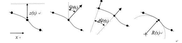
Figure 2.1: Measurement of position, slope, slope difference and curvature
2.1 Conceptual considerations
Measuring position (i.e. surface coordinates) gives similar measurement versatility as current CMMs. It allows for true universal measurement, also for discontinuous parts, reference markers and quick alignment checks. Further, each individual measurement point can be directly traced back to a point on the surface, which is not the case when measuring other measurands.
Optically measuring distance is relatively difficult. It generally requires a spot to be focused onto the surface. To obtain high axial resolution, a high NA and thus a small spot (micrometer order) is necessary. This makes it very sensitive to local defects. Furthermore, measuring position requires the position of the sensor relative to the product to be known at similar accuracy level, which yields high requirements for the scanning system.
Slope can optically be measured relatively easily and accurately, for instance with a deflectometer (miniature autocollimator). In (Szwedowicz, 2006) remarkable results have been obtained in wafer measurement, also because of a multi-path integration algorithm that suppresses random measurement errors. The spot size can range from 0.1 - 1 mm, which makes it relatively insensitive to local surface defects. With this setup nanometer height resolution has been shown for wafer measurements.
There also are some disadvantages. First of all, due to the required integration of the data, discontinuous surfaces (such as multiple optical surfaces on one part or reference markers on the product carrier) can not be measured. To reconstruct a surface, a high density data set is always required. A quick check to confirm coarse surface form or alignment for instance by measuring some specific points on the surface, is thus not possible.
Due to the slope measurement, the positioning requirements of the sensor relative to the product are somewhat relieved, but the angular position of the sensor is still critical to prevent systematic integration errors. Because the distance between the surface and the sensor is not known, the actual point of measurement in space is difficult to determine, which leads to uncertainties for the absolute dimensions and location of the part (radius of curvature, diameter etc.), especially for strongly curved parts.
Instead of measuring slope, the slope difference between two points (Geckeler and Weingärtner, 2002) or the local curvature at a point (Schulz and Weingärtner, 2002) can also be measured. These properties are intrinsic properties of a surface, which can be measured independently of the object’s orientation relative to an outside reference. This relieves the positioning requirements of the sensor relative to the product. By dual integration, the surface form can be calculated. Due to the required integration, these methods suffer from the same disadvantages as slope measurement. Further, curvature ranges from convex to concave with local radii of curvature down to some tens of millimeters. No curvature sensor yet has sufficient dynamic range to universally satisfy these demands. The curvature sensor commonly used is a miniature interferometer using a CCD, which does not allow for continuous scanning.
Traceability
The measurand of choice also depends on the traceability. Traceability can be provided by either verifying the process with a large series of reference artefacts that cover the range of products to be measured, or by characterizing the grouped or individual elements of the entire metrology loop of the instrument. Besides tilted flats and off-axis spheres, no true freeforms calibrated to the required uncertainty are yet available (Savio et al., 2007). Hence, the metrology loop will have to be characterized. When measuring positions, this is relatively straightforward since each individual measurement can be directly traced to a point on the surface. Further, measuring form from position data is standard practice at the National Metrology Institutes.
When measuring slope, slope difference or curvature, the individual measurements can be calibrated using autocollimators, angle gauges or reference spheres. Correct individual measurements do not necessarily guarantee that the reconstructed form is correct due to the data integration. Proving traceability of this process is thus less straightforward since it is dependent on the entire slope data set.
Regarding the above, measuring position is believed to result in the most versatile and traceable measurement method. Therefore, a distance measuring optical probe will be scanned over the surface.
Setup
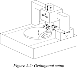
To position the probe over the surface, an orthogonal, cylindrical or polar setup can be used. Conventional coordinate measurement machines use an orthogonal setup as shown in Figure 2.2. The probe is translated in 3 directions (x, y and z). To orient the probe perpendicular to the surface, this setup can be extended with two rotations (ϕandψ). For high speed scanning all axes are thus continuously in motion resulting in large moving masses and accelerations. The 3 translations and 2 rotations further result in a fully 3D metrology loop. The required strokes are approximately 700 x 700 x 150 mm and rotations up to 180° depending on the chosen rotation axis setup.
2.1 Conceptual considerations
Since the surfaces are more or less rotationally symmetric (within 5 mm PV), a cylindrical setup appears to be the obvious choice. The product can be mounted on a continuously rotating spindle (θ), while the probe is positioned in radial (r) and vertical (z) direction. To align the probe to the global surface slope, one rotation (ψ) is required. Here, the spindle can be rotating continuously, while the probe is positioned over the surface in circular or spiral tracks. The stages move in small slow steps, so system dynamics is improved compared to the orthogonal setup. Due to the large difference between the displacement in the plane of motion and perpendicular to it, the metrology loop generally referred to as 2½D.
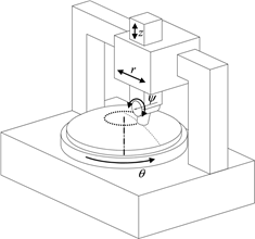
Figure 2.3: Cylindrical setup
The surfaces are not only more or less rotationally symmetric; they will also be more or less spherical. A polar or swing arm setup (Figure 2.4) might therefore also be applied (Anderson and Burge, 1995; Callender et al., 2006). When the rotation axis of the arm coincides with the centre of curvature of the surface, the entire surface can be measured with only two rotations (ζ and θ). The probe inherently stays perpendicular with the best-fit-sphere of the surface. This setup also allows for fast scanning of circular tracks.
When measuring different radii of curvature (especially with changing from convex to concave), the inclination angle of the bearing of the arm has to be adjusted. Also, for small radii, in the order of several tens of millimeters, the physical dimensions of the arm and bearing become a problem. Due to the required adjustments, this setup is thus not universal. Aligning the rotation axis and the probe to the (non-physical) centre of curvature of the surface is difficult, especially when the surface is nonspherical. This leads to uncertainty in the absolute surface dimensions and position. Further, the influence of gravity on the arm is continuously changing, and the metrology problem for this setup is fully 3D again. Provided that calibration issues are resolved, this setup is more suitable for near constant radius measurements of large series of large surfaces.
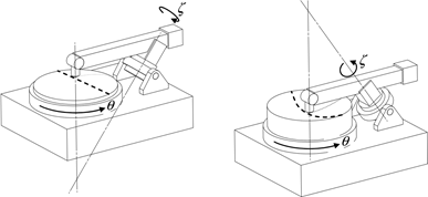
Figure 2.4: Polar setup for convex and concave surfaces
Concluding from the above, the cylindrical setup of Figure 2.3 is the obvious choice. It is truly universal, can be fast with relatively little system dynamics, uses only four axes of motion and it has a 2½ D metrology loop.
Stage layout
Some variations are possible to the cylindrical setup of Figure 2.3, similarly to the considerations of (Vermeulen, J., 1999). The spindle can be oriented vertically and horizontally. The vertical orientation is preferred due to the large product mass and diameter of 500 mm. This way the accessibility and visibility for loading, aligning and fixing of a product is most convenient. Further the spindle is loaded axially, preventing mass dependent bending forces and eccentricity of the spindle rotor. The ψ-rotation can best be done with the probe, since it is the smallest mass and thus is least affected by the changing direction of gravity. The remaining 2 translations (r and z) can be performed with the spindle, the probe or a combination of the two. Due to the large spindle and product mass (~200 kg), moving the lightest component (i.e. the probe) will result in the best dynamic behaviour. Furthermore, this setup will lead to the shortest metrology loop as will be shown in Chapter 4. The cylindrical setup of Figure 2.3 is thus the preferred stacking sequence of the stages.
2.2 Machine concept
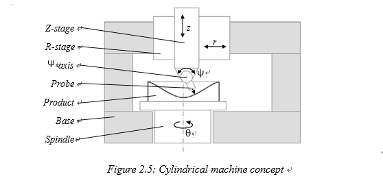
The chosen cylindrical concept is shown in Figure 2.5. The product is mounted on an air-bearing spindle, which is rotating continuously at for instance 1 rev/s. An optical distance probe is mounted on a rotation axis (Ψ-axis) which positions it perpendicular to the rotationally symmetric best-fit of the product. The probe can be moved in radial and vertical direction by an R and Z-stage, respectively.
2.2 Machine concept
The probe will be positioned on a circular track on the product and the stages will be locked. This improves the positioning stability of the stages since the electronic noise of the motors and encoders is cancelled. The track can be measured multiple times with little extra effort, to obtain redundant data, for instance for averaging. After this, the stages are moved about 1 mm further to the next track and the process is repeated. This allows for measurement times in the order of 15 minutes for large surfaces.
When a freeform surface is rotating on the spindle, the surface may vary between the continuous and dotted line in Figure 2.6 by 5 mm PV. As will be explained in Chapter 5, optical probes generally only have a focal depth of a few micrometers. Keeping the probe in focus by actuating the R and Z-stage requires large accelerations of these heavy stages, resulting in undesirable dynamics. To avoid this, a probe with 5 mm range is required. This way the stages can be held stationary even when measuring a freeform track. This reduces the dynamically moving mass from a few hundred kg for the stages to only 50 g of the probe objective. This improves system dynamics and allows for maintained high scanning speed for freeforms surfaces.

The total measurement uncertainty is composed of many factors, such as probe position, product position, probe-surface interaction, form stability of the surface under test, the data-acquisition and the data-processing software.
The largest contribution is expected to be determined by the metrology loop between the probe and the product. In Figure 2.5, this loop was equal to the structural loop and thus included the stages, bearings, base etc. By applying a metrology frame relative to which the probe and product position are measured as directly as possible, most stage errors can be eliminated from the metrology loop, as shown in Figure 2.6.
The spindle is intended to rotate at 1 rev/s. The worst case deformation of the surface under test due to the centrifugal force was estimated using FEM for a ∅500 mm flat, concave and convex surface with material properties similar to aluminium or glass. Depending on the boundary conditions (e.g. fixed backside, three-point mount, fixed centre), the deformation varied between 3 and 40 nm. Part of this deformation is of the less-sensitive type (see section 2.3.2). by modelling the effect in FEM, this deformation can be compensated for in the data-processing.
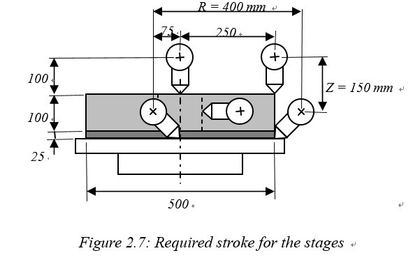
The required stroke is shown in Figure 2.7. The length of the probe is 100 mm. To be able to orient the probe at + and –45° throughout the measurement volume, the range of the R-stage has to be 400 mm (–75 to +325 mm), and range of the Z-stage has to be 125 mm. To optionally incorporate an intermediate body as a product carrier, the Zstage range is further increased to 150 mm. It is further convenient to have a ψ-range of –45° to +120° for calibration and nulling purposes, as further explained in section 7.3.
This concept can meet the design goals. The Ψ-axis enables application of an optical probe. By increasing the measurement range of this probe to 5 mm and combining it with a cylindrical machine setup, freeforms can be measured universally with high scanning speeds and minimal dynamics. The separate 2D metrology loop somewhat
2.2 Machine concept
relieves the requirements on the structural loop. Due to the non-contact nature, measurement is more important than actual positioning. This may allow for achieving the desired uncertainty.
2.3 Error budget
2.3.1 Coordinate system definition
To emphasize the cylindrical nature of the machine, an r,y,z coordinate system has been adopted (Figure 2.8). The origin of the system is located at the spindle surface centre, the z-direction is coaxial with the spindle centre line and the r-direction (‘radial’) is parallel to the plane of motion of the probe. This plane is also referred to as the ‘measurement plane’. The rotations around the r, y and z axis are ϕ, ψ and θ, respectively.
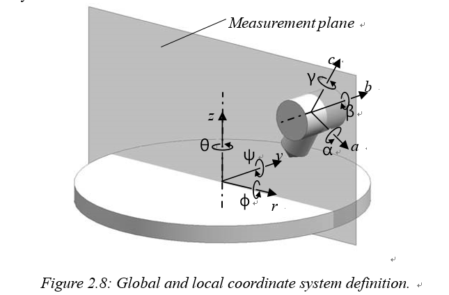
As will become clear, it is convenient to also define a local coordinate system that rotates with the probe. In this system, the c-direction is aligned with the probe axial direction and the b-direction is parallel to the y-direction of the global coordinate system. Rotations around the a, b and c axes are called α, β and γ, respectively. The β-direction coincides with the ψ-direction. The origin is located at the Ψ-axis centre line.
2.3.2 Error sensitivity
The probe is aligned to the rotationally symmetric best-fit of the surface. When measuring a flat, sphere or asphere, the probe will always be nominally perpendicular to the surface, and the local curvature and slope equal the global curvature and slope. With freeform surfaces, the 5 mm PV departure from rotationally symmetry inherently results in a departure of local slope and curvature from global values. Since the probe will not be actively controlled perpendicular to the surface during the measurement of an individual track, the local slope variations cause a misalignment between probe and surface in α as well as β direction of up to 5° (see section 1.1.3).
The metrology loop is composed of three main elements: the distance measured by the probe, the measured position of the probe relative to the metrology frame and the measured position of the product relative to the metrology frame. To model the sensitivity of errors in these three elements, they are interpreted as displacements of the probe relative to the product. The error in the distance measured by the probe as a result of this displacement δ is the measurement error Δ..
As illustrated in Figure 2.9 A, a distance measurement error of the probe, and a position measurement error n with its resulting vector in normal direction n of the surface, both result in a direct measurement error n.
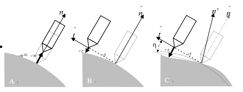
Figure 2.9: Distance measurement error resulting from displacement in normal (n) and tangential (t) direction.
A position measurement error t in tangential direction t of the surface, results in an error c that is dependent on local surface geometry. Since the surfaces are smoothly curved and have low roughness, only local curvature and tilt have to be taken into account here. When measuring rotationally symmetric surfaces (flats, spheres and aspheres), the probe is always nominally perpendicular to the surface (Figure 2.9 B). Therefore only local curvature can cause an error here. A position measurement error in tangential direction only results in a second order error c. Figure 2.10 (left) shows this error up to an Rc of 10 mm and a t of 2 μm, to be only 0.2 nm. Errors due to local curvature are thus negligible.
2.3 Error budget
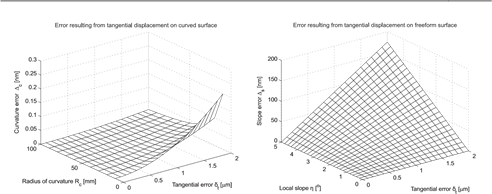
Figure 2.10: Error as a function of curvature (left) and local slope (right)
Local surface slopes of 5° are expected (section 1.1.3), which is also the maximum misalignment between probe and surface (Figure 2.9 C). The resulting distance measurement error is linearly dependent to this local slope, as shown in Figure 2.10 (right). This error can be substantial for large local slopes and large tangential errors. A sub-micrometer out-of-plane error is therefore desirable.
One may argue that the probe therefore is to be kept perpendicular to the local surface slope to avoid these errors. This would require the probe to be rotated around its tip while measuring a track, preferably with a virtual pivot at the probe tip. This would add two new stages to the system that have to be actuated and measured. Moreover, the motion system currently is a 2D system, which allows for direct 2D metrology to the probe as will be shown in Chapter 4. Adding the virtual pivot would turn the metrology system back to fully 3D, significantly increasing the complexity and the measurement uncertainty of the system. Local surface slope is expected to be below a few tenths of a degree for most surfaces. A 2D system is therefore designed, and the higher measurement uncertainty for a minority of highly complex freeform surfaces is accepted.
When the sensitivity of 0.087 is compared to the sensitivity of 1 for errors in normal direction, over an order of magnitude reduced sensitivity to tangential errors is seen. For surfaces with less local slope, this reduction is even better. A clear distinction between normal and tangential errors can thus be concluded.
With the metrology frame as a reference, 13 degrees of freedom can be distinguished. These are the 6 DOFs of the product, plus the 6 DOFs of the probe, plus the distance measured by the probe. For each of these, the resulting error (normal and/or tangential) between probe and product can be calculated as a function of position measurement error and surface geometry. Further, the measurement position has to be taken into account. When measuring a flat surface for instance, a radial error has no influence, and tilting of the product linearly influences the measurement error as a function of the radial measurement position. The resulting measurement error will thus be measurement-task specific.
As explained in Figure 2.10, the errors resulting from tangential errors on a curved surface are negligible. For aspheres, the measurement uncertainty is therefore predominantly determined by errors in normal direction. Only six degrees of freedom cause errors in normal direction, as shown in Figure 2.11. These degrees of freedom determine the basic measurement uncertainty for aspheres and mild freeforms, and are called the ‘sensitive directions’. The other seven directions are referred to as the ‘lesssensitive’ directions.

Figure 2.11: Degrees of freedom that result in a displacement between probe and surface in normal direction, i.e. the sensitive directions.
2.3.3 Error budget
When the error sources of the 13 individual degrees of freedom are assumed uncorrelated and normally distributed, the resulting uncertainty in a, b and c direction can be calculated with (2.1). Here, σi,j is the rms error of part i in direction j, where the part is the spindle (S) or the probe (P). The probe angle is ψ, R and Z are the probe tip position and LP is the length of the probe.
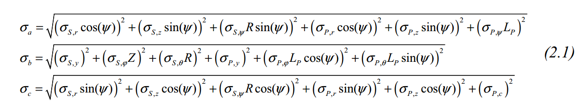
The uncertainty in normal direction is equal to the uncertainty in c-direction, while the uncertainty in tangential direction is the resulting vector of the a and b-direction:
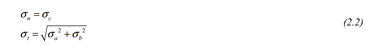
If we assume that the normal and tangential uncertainties are uncorrelated for the sake of simplicity, this makes the total uncertainty equal to quadratic sum of the normal uncertainty plus the tangential uncertainty times the local resulting slope η:

The error budget was iteratively divided over the individual components, with the somewhat arbitrary resulting maximum budgeted error (3σ) per DOF, relative to the metrology frame, as shown in Table 2.1. The spindle error budget is based on vendor specifications and error motion measurement literature, as further discussed in sections 3.3.5 and 4.4. The error budget for the probe position is based on design and calibration literature, as explained throughout Chapter 3 and Chapter 4. The error budget for the probe is based on a literature study as shown in Chapter 5 and Appendix I.
The six critical error directions are marked in gray; the other seven directions determine the magnitude of the less sensitive tangential error. Due to their reduced sensitivity, these can be allowed to be an order of magnitude larger than the errors in normal direction.

With the maximum error values chosen as shown in Table 2.1, the resulting form measurement uncertainty is shown in Figure 2.12. The uncertainty is task-specific, but is mainly dependent on the diameter of the part and the local slope. Figure 2.12 was calculated with ψ = 22.5°, Z = 50 mm and a probe length LP of 100 mm. The gray area at the base plane shows the surfaces for which the 30 nm expanded uncertainty objective is met. The uncertainty increases to 55 nm for heavily freeform surfaces.
The values of Table 2.1 are the allowed maximum errors relative to the metrology frame, after calibration. The sensitive directions (in gray) are certainly challenging, and will be measured by the metrology loop. The other seven less-sensitive directions are also challenging, but are thought to be possible with the structural loop alone. The machine concept can thus be split into two parts: a 2D metrology loop that measures the position of the probe relative to the product within the measurement plane at nanometer level, and a structural loop that mechanically provides a sub-micrometer accuracy plane of motion for the probe relative to the product after calibration.
2.4 Machine design overview
2.4.1 Main design aspects
An overview of the main concepts that have been applied in the machine design is given in the following section, to aid better understanding of the detailed subsystem designs in the coming chapters.
Structural loop
The structural loop should provide a high accuracy plane of motion to the probe. To achieve this, the Z-stage is directly aligned to a vertical plane of the base using three air bearings. This provides higher out-of-plane accuracy, stiffness and stability compared to a stacked design.

Figure 2.13: Z-stage with 3 bearings to a vertical plane
To minimize distortions and hysteresis, separate preload and position frames will be applied in both the R and Z-stage. Due to the cylindrical setup and the long range probe, the stages can be stationary while measuring a circular track. To increase the stiffness and stability of the stages in the actuated directions, mechanical brakes will be applied that clamp the stages. This prevents stage motion from encoder, amplifier and EMC noise, and may provide higher stiffness compared to the achievable servo
2.4 Machine design overview
stiffness. Only the degree of freedom in the motion direction of the stage will be clamped to prevent stage deformation.
Metrology loop
To satisfy the Abbe principle, the measurement systems should be aligned to the probe focal point. When measuring concave optics, however, the edge of the optic is blocking the horizontal line of sight between the outside reference and the probe focal point. Moreover, the vertical and horizontal position of the probe focal point changes with ψ-rotation, whilst the stages remain stationary. This would require a metrology system that tracks the probe-tip position independently of the stage position.
The setup is less-sensitive to tangential errors of the probe focal point relative to the product. As shown in the error budget calculations, this also includes the ψ-rotation of the probe. The Abbe point can therefore be shifted from the probe focal point to the Ψ-axis centre. The measurement systems can now be aligned with the Ψ-axis centre, and move along with the R and Z-stages. Due to the reduced tangential sensitivity, the Abbe principle is still satisfied.
To measure the displacement of the Ψ-axis rotor (1 in Figure 2.14) relative to the metrology frame (2), an interferometry system is applied. Hereto the Ψ-axis rotor has been made reflective such that the measurement beam (3) can be focused onto it by a lens (4). The beam layout is such that the measurement beam also reflects on a reference mirror (5), directly measuring the displacement between the Ψ-axis rotor and the reference mirror. A similar setup is employed in horizontal direction (6). Reaction forces of the probe servo system (7) on the Ψ-axis bearing, or pressure variations in the stage bearings will cause displacement of the probe. With this setup, the position errors of the whole motion system in r- and z-direction are measured at the Ψ-axis rotor, and can be compensated for in the data-processing.
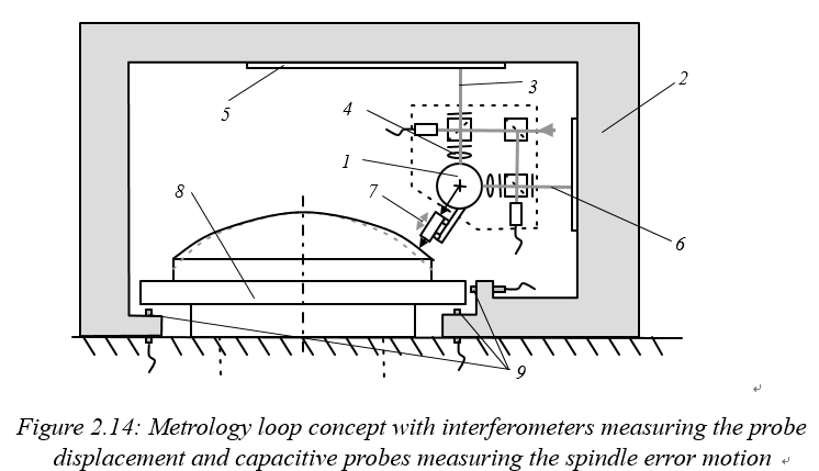
Although the acquired spindle (8) is specified to have an error motion of only 25 nm and 0.1 μrad, the position of the rotor needs to be determined to 15 nm and 0.1 μrad. To determine the position of the spindle rotor relative to the metrology frame, capacitive probes (9) are therefore added. Principally, three capacitive probes are sufficient to measure the three sensitive directions r, z and ψ. Seven probes are however applied, to separate the roundness error from the error motion with the multiprobe method.
The displacement of the probe and spindle are measured relative to the metrology frame. This frame is constructed out of Silicon Carbide. The high specific stiffness results in high eigenfrequencies, and the high thermal diffusivity combined with low expansion coefficient minimize the sensitivity to thermal gradients. Further, the material is hard enough to polish the reference mirrors directly onto the beams, avoiding separate strip mirrors of limited stiffness and stability and connection elements.
With this metrology loop concept, all six sensitive directions of Figure 2.11 are measured directly. When measuring a freeform surface, only the probe focusing mechanism is moving dynamically while measuring a circular track. The static and dynamic displacements that occur during this measurement are recorded by the metrology system and can be compensated for in the (off-line) data-processing.
Non contact probe
A two stage probe has been designed (Figure 2.15). The short stroke differential confocal principle measures the absolute distance to the surface, with a range of a few micrometers. This short stroke system is mounted on a linear guidance that is servocontrolled to keep the surface in range. The required displacement of the short stroke system is measured with the long stroke system. Incremental systems, such as an interferometer or optical encoder, can provide the required dynamic range here since this measurement no longer has to be absolute. The distance measured by the probe is the sum of the short and long stroke outputs.

2.4.2 Machine design overview
The final machine design is shown in Figure 2.16. It measures 2.1 m wide, 1.85 m deep and 1.8 m high. The total mass is approximately 3500 kg.

Figure 2.16: Machine design overview
The machine design consists of three main systems: the motion system, the metrology system, and the non-contact probe (Figure 2.17). These will be discussed in detail in Chapters 3 to 5. The fourth subsystem is the electronics and software, which will be discussed in Chapter 6. The complete machine assembly and validation experiments are discussed in Chapter 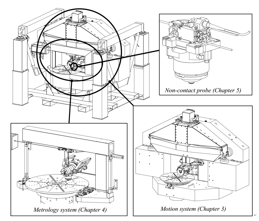
Figure 2.17: Main subsystems