上篇文章介绍了Diffusion扩散模型的原理,这篇文章以此为基础,努力学会StableDiffusion的原理和实现。
原理部分参考大佬的文章,原理从文字和图来看并不复杂,但是当你亲自去实现的时候,就会发现这是一件多么困难的事情,入门易,下手难呀!
Stable Diffusion原理解读 - 知乎 (zhihu.com)

从SD论文的架构图中,就可以明显看出SD于Diffusion模型的改进之处,
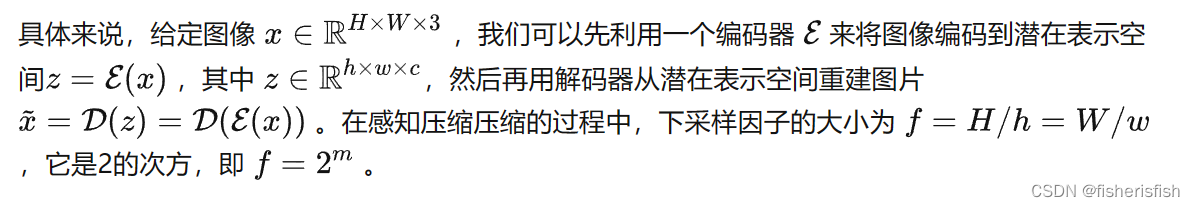
1、首先,SD增加了图片感知压缩(Perceptual Image Compression),也就是左边的红框区域。
图片感知压缩(Perceptual Image Compression)
简单来说,就是原本diffusion模型直接在像素层面训练,内存占用太大,引入感知压缩就是说通过VAE这类自编码模型对原图片进行处理,忽略掉图片中的高频信息,只保留重要、基础的一些特征。这种方法带来的的好处就像引文部分说的一样,能够大幅降低训练和采样阶段的计算复杂度,让文图生成等任务能够在消费级GPU上,在10秒级别时间生成图片,大大降低了落地门槛。
感知压缩主要利用一个预训练的自编码模型,该模型能够学习到一个在感知上等同于图像空间的潜在表示空间。这种方法的一个优势是只需要训练一个通用的自编码模型,就可以用于不同的扩散模型的训练,在不同的任务上使用。这样一来,感知压缩的方法除了应用在标准的无条件图片生成外,也可以十分方便的拓展到各种图像到图像(inpainting,super-resolution)和文本到图像(text-to-image)任务上。
由此可知,基于感知压缩的扩散模型的训练本质上是一个两阶段训练的过程,第一阶段需要训练一个自编码器,第二阶段才需要训练扩散模型本身。在第一阶段训练自编码器时,为了避免潜在表示空间出现高度的异化,作者使用了两种正则化方法,一种是KL-reg,另一种是VQ-reg,因此在官方发布的一阶段预训练模型中,会看到KL和VQ两种实现。在Stable Diffusion中主要采用AutoencoderKL这种实现。
2、由于进行了图像编码,所以原来的diffussion model变成了latent diffusion model
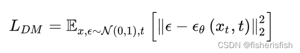

LDM就是上一篇文章得到的DM的损失函数,这里变成了LLDM,就是讲输入变成了latent的输入,Zt为编码器得到的结果。
3、最后便是SD引入了Conditioning Mechanisms,也就是输入文本等约束生成特定的图像,从图中可以看出,条件约束通过引入了一个领域专用编码器(domain specific encoder)![]()
并且是在diffusion的逆向推理过程的Unet中增加了cross-attention机制来实现![]()
简单来说就是加了一个transformer里的一个自注意力机制Q是原Zt,K和V由条件输入决定,损失函数变成了LLDM
 Stable Diffusion 原理介绍与源码分析(一) - 知乎 (zhihu.com)
这里我们从三个模块的源码开始学习
首先是Encode_First_Stage,也就是将图像映射到隐藏层,这里引用珍妮大佬的图 说明这个过程发生了什么

在SD源码中,位于img2img.py下,有以下代码调用此过程
    init_image = load_img(opt.init_img).to(device)
    init_image = repeat(init_image, '1 ... -> b ...', b=batch_size)
    init_latent = model.get_first_stage_encoding(model.encode_first_stage(init_image))  # move to latent space
而在最新版的SD中其默认的推理config为
    parser.add_argument(
        "--config",
        type=str,
        default="configs/stable-diffusion/v2-inference.yaml",
        help="path to config which constructs model",
    )
在此config中,我们可以找到该层相关参数
    first_stage_config:
      target: ldm.models.autoencoder.AutoencoderKL
      params:
        embed_dim: 4
        monitor: val/rec_loss
        ddconfig:
          #attn_type: "vanilla-xformers"
          double_z: true
          z_channels: 4
          resolution: 256
          in_channels: 3
          out_ch: 3
          ch: 128
          ch_mult:
          - 1
          - 2
          - 4
          - 4
          num_res_blocks: 2
          attn_resolutions: []
          dropout: 0.0
        lossconfig:
          target: torch.nn.Identity
加载模型的代码如下,可见模型是通过ldm.util中的instantiate_from_config函数加载的
from ldm.util import instantiate_from_config
def load_model_from_config(config, ckpt, verbose=False):
    print(f"Loading model from {ckpt}")
    pl_sd = torch.load(ckpt, map_location="cpu")
    if "global_step" in pl_sd:
        print(f"Global Step: {pl_sd['global_step']}")
    sd = pl_sd["state_dict"]
    model = instantiate_from_config(config.model)
    m, u = model.load_state_dict(sd, strict=False)
    if len(m) > 0 and verbose:
        print("missing keys:")
        print(m)
    if len(u) > 0 and verbose:
        print("unexpected keys:")
        print(u)

    model.cuda()
    model.eval()
    return model
这里我们直接找到ldm.model中的autoencoder.py,即可找到这一层的源码,然后我们直接找到AutoencoderKL中的前向代码,可见其就是将输入编码然后解码,返回编解码结果dec和一个posterior
    def forward(self, input, sample_posterior=True):
        posterior = self.encode(input)
        if sample_posterior:
            z = posterior.sample()
        else:
            z = posterior.mode()
        dec = self.decode(z)
        return dec, posterior
其encode和decode代码如下,其中最关键的encoder和decoder引用ldm.modules.diffusionmodules.model
from ldm.modules.diffusionmodules.model import Encoder, Decoder
    def encode(self, x):
        h = self.encoder(x)
        moments = self.quant_conv(h)
        posterior = DiagonalGaussianDistribution(moments)
        return posterior

    def decode(self, z):
        z = self.post_quant_conv(z)
        dec = self.decoder(z)
        return dec
这里简单介绍一下AutoencoderKL,它来自Auto-Encoding Variational Bayes(VAE)这篇论文
AutoencoderKL (huggingface.co)
Auto-Encoding Variational Bayes(VAE) - 知乎 (zhihu.com)
Auto encoder是一种无监督算法,主要用于特征提取或数据降维。其思想非常简单,即输入特征X 经过encoder后抽象为hidden layer z,再将z经过decoder过程重新预测为。

Auto encoder的目的是提取抽象特征z,其学习过程为最小化损失函数,
用于惩罚二者之间的差异,假设使用平方损失,则有:
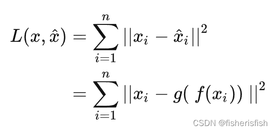
所以个人猜测AutoencoderKL实际上是用KL散度作为损失函数的AE,不知道对不对哈
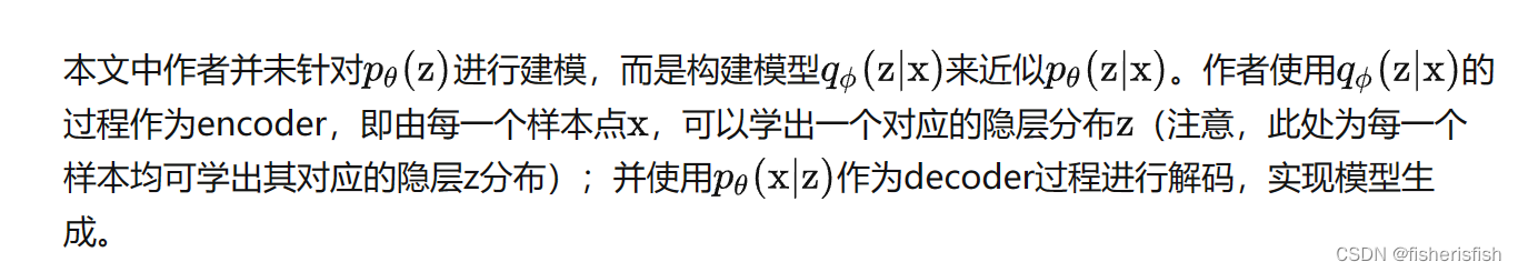
VAE的目的:很多时候,当我们数据处理时,会遇到数据量不足的情况,这时我们会考虑使用生成模型生成数据。VAE即在AE的基础上引入变分的思想,使其能够进行数据生成。
而其思路是试图推断和学习有向概率图模型的隐分布z,并通过对z的采样来实现数据生成。
这里直接引用慕容三思大佬的原文,大佬文章真的写得非常通俗易懂

这里其实和diffusion模型有些类似,具体过程应该是先通过encoder获得隐分布z,然后用类似扩散模型的方法生成,然后计算输入输出的KL散度,调整decoder
 而具体计算的过程也和Diffusion类似,yysy,VAE应该比diffusion早?所以应该是diffusion借鉴了VAE?
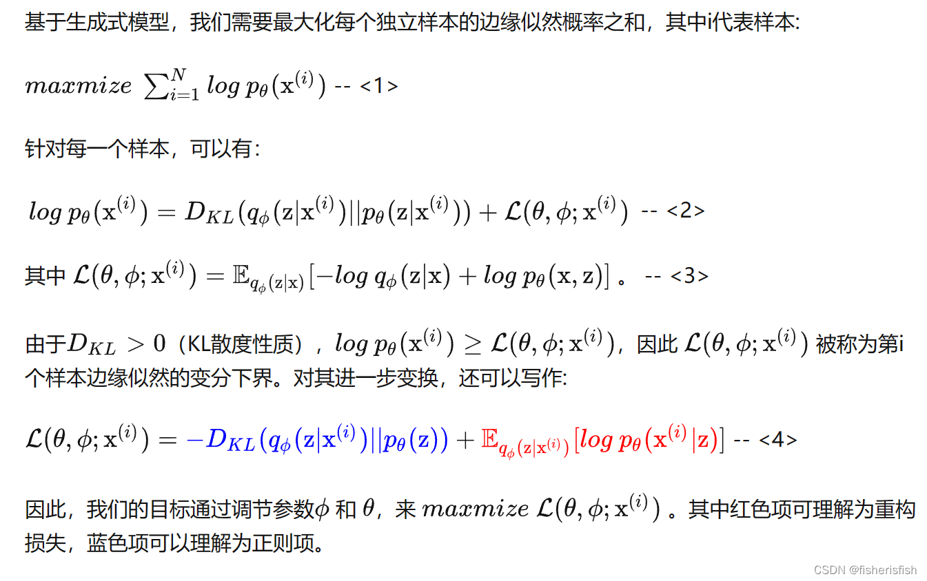
然后是和diffusion类似的损失函数推理过程,同样使用了KL散度计算二者之间的差异,然后我也终于进一步看懂了损失函数的意义,最大化每个独立样本的边缘似然概率之和。而每一个样本的差异则是通过KL散度计算两个分布的差异和一个额外的损失函数构成
这里要看懂还是得多学习概率论计算才行
这个过程在具体实现时同样需要The reparameterization trick(重参数化)


VAE的具体步骤如下
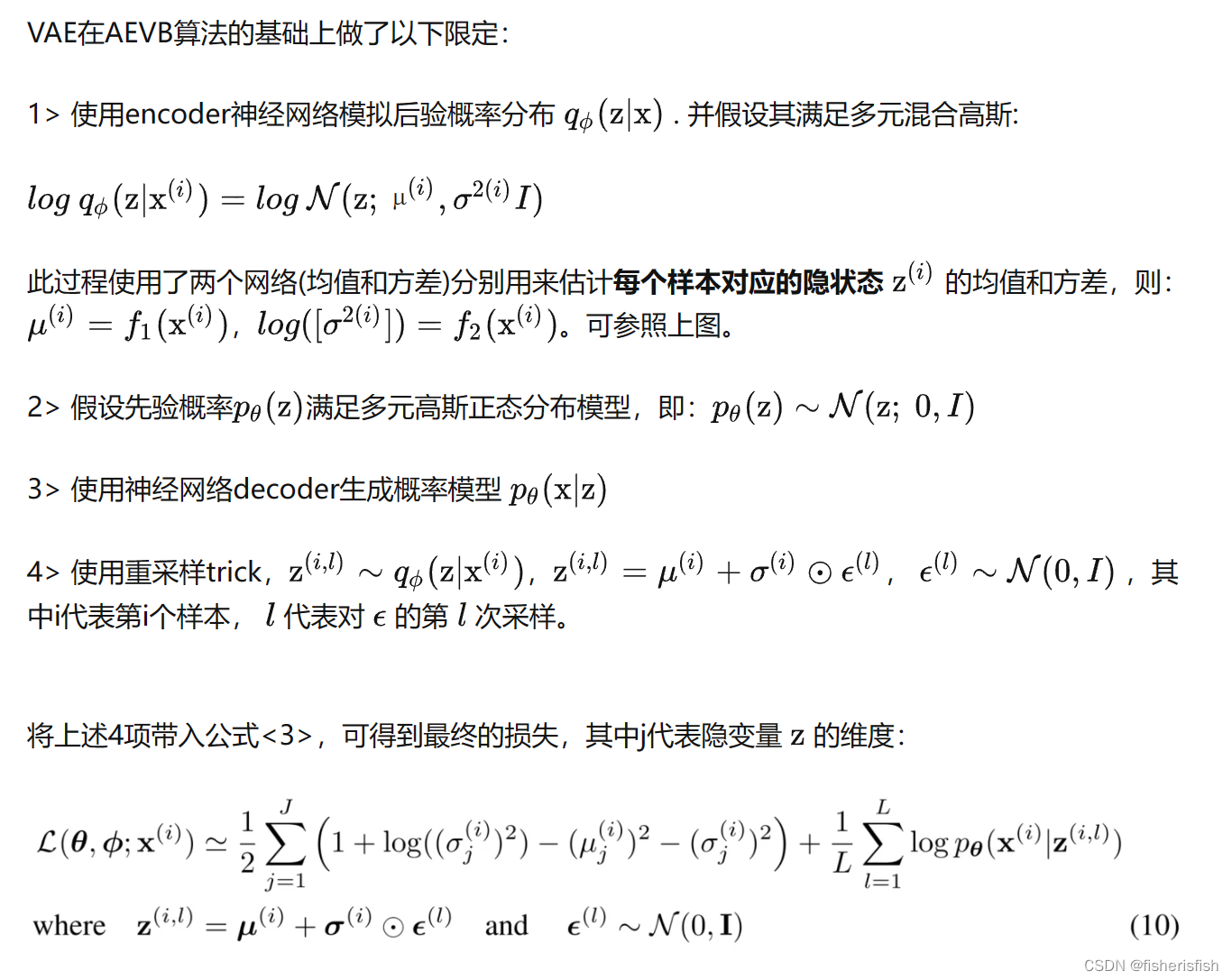
接着我们来看一下AEKL的代码实现
    def encode(self, x):
        h = self.encoder(x)
        moments = self.quant_conv(h)//self.quant_conv = torch.nn.Conv2d(2*ddconfig["z_channels"], 2*embed_dim, 1)
        posterior = DiagonalGaussianDistribution(moments)
        return posterior

    def decode(self, z):
        z = self.post_quant_conv(z)//self.post_quant_conv = torch.nn.Conv2d(embed_dim, ddconfig["z_channels"], 1)
        dec = self.decoder(z)
        return dec

    def forward(self, input, sample_posterior=True):
        posterior = self.encode(input)
        if sample_posterior:
            z = posterior.sample()
        else:
            z = posterior.mode()
        dec = self.decode(z)
        return dec, posterior
在AEKL的forward过程中,先进行encode编码,再进行sample取样,最后再进行解码,解码部分在SD中并不是跟着编码过程后马上进行的,而是在隐式空间内进行了diffusion操作,所以decoder部分放在后面来讲,我们来看encode具体做了什么:encode同样分三步,第一步是encoder中用多个resnet进行特征提取,然后是quant_conv进一步调整通道数,最后是DiagonalGaussianDistribution计算特征分布的均值、方差、标准差等
Encoder的前向推理步骤如下
    def forward(self, x):
        # timestep embedding
        temb = None

        # downsampling
        hs = [self.conv_in(x)]//self.conv_in = torch.nn.Conv2d(in_channels,self.ch,kernel_size=3,stride=1,padding=1),一个简单的3*3卷积
        for i_level in range(self.num_resolutions)://self.num_resolutions = len(ch_mult),ch_mult=(1,2,4,8),应该是指降采样的次数,ch_mult是降采样的倍数
            for i_block in range(self.num_res_blocks)://self.num_res_blocks = num_res_blocks,来自于输入,在config文件中设置值为2
                h = self.down[i_level].block[i_block](hs[-1], temb)
                if len(self.down[i_level].attn) > 0:
                    h = self.down[i_level].attn[i_block](h)
                hs.append(h)
            if i_level != self.num_resolutions-1:
                hs.append(self.down[i_level].downsample(hs[-1]))

        # middle
        h = hs[-1]
        h = self.mid.block_1(h, temb)
        h = self.mid.attn_1(h)
        h = self.mid.block_2(h, temb)

        # end
        h = self.norm_out(h)
        h = nonlinearity(h)
        h = self.conv_out(h)
        return h
self.down的定义如下,可见其是由ResnetBlock和attn构成的,而v2-inference版本没有用注意力,所以此处的down部分仅有多个ResnetBlock构成
        self.down = nn.ModuleList()
        for i_level in range(self.num_resolutions):
            block = nn.ModuleList()
            attn = nn.ModuleList()
            block_in = ch*in_ch_mult[i_level]
            block_out = ch*ch_mult[i_level]
            for i_block in range(self.num_res_blocks):
                block.append(ResnetBlock(in_channels=block_in,
                                         out_channels=block_out,
                                         temb_channels=self.temb_ch,
                                         dropout=dropout))
                block_in = block_out
                if curr_res in attn_resolutions:
                    attn.append(make_attn(block_in, attn_type=attn_type))
            down = nn.Module()
            down.block = block
            down.attn = attn
            if i_level != self.num_resolutions-1:
                down.downsample = Downsample(block_in, resamp_with_conv)
                curr_res = curr_res // 2
            self.down.append(down)

//self.down
ModuleList(
  (0): Module(
    (block): ModuleList(
      (0-1): 2 x ResnetBlock(
        (norm1): GroupNorm(32, 128, eps=1e-06, affine=True)
        (conv1): Conv2d(128, 128, kernel_size=(3, 3), stride=(1, 1), padding=(1, 1))
        (norm2): GroupNorm(32, 128, eps=1e-06, affine=True)
        (dropout): Dropout(p=0.0, inplace=False)
        (conv2): Conv2d(128, 128, kernel_size=(3, 3), stride=(1, 1), padding=(1, 1))
      )
    )
    (attn): ModuleList()
    (downsample): Downsample(
      (conv): Conv2d(128, 128, kernel_size=(3, 3), stride=(2, 2))
    )
  )
  (1): Module(
    (block): ModuleList(
      (0): ResnetBlock(
        (norm1): GroupNorm(32, 128, eps=1e-06, affine=True)
        (conv1): Conv2d(128, 256, kernel_size=(3, 3), stride=(1, 1), padding=(1, 1))
        (norm2): GroupNorm(32, 256, eps=1e-06, affine=True)
        (dropout): Dropout(p=0.0, inplace=False)
        (conv2): Conv2d(256, 256, kernel_size=(3, 3), stride=(1, 1), padding=(1, 1))
        (nin_shortcut): Conv2d(128, 256, kernel_size=(1, 1), stride=(1, 1))
      )
      (1): ResnetBlock(
        (norm1): GroupNorm(32, 256, eps=1e-06, affine=True)
        (conv1): Conv2d(256, 256, kernel_size=(3, 3), stride=(1, 1), padding=(1, 1))
        (norm2): GroupNorm(32, 256, eps=1e-06, affine=True)
        (dropout): Dropout(p=0.0, inplace=False)
        (conv2): Conv2d(256, 256, kernel_size=(3, 3), stride=(1, 1), padding=(1, 1))
      )
    )
    (attn): ModuleList()
    (downsample): Downsample(
      (conv): Conv2d(256, 256, kernel_size=(3, 3), stride=(2, 2))
    )
  )
  (2): Module(
    (block): ModuleList(
      (0): ResnetBlock(
        (norm1): GroupNorm(32, 256, eps=1e-06, affine=True)
        (conv1): Conv2d(256, 512, kernel_size=(3, 3), stride=(1, 1), padding=(1, 1))
        (norm2): GroupNorm(32, 512, eps=1e-06, affine=True)
        (dropout): Dropout(p=0.0, inplace=False)
        (conv2): Conv2d(512, 512, kernel_size=(3, 3), stride=(1, 1), padding=(1, 1))
        (nin_shortcut): Conv2d(256, 512, kernel_size=(1, 1), stride=(1, 1))
      )
      (1): ResnetBlock(
        (norm1): GroupNorm(32, 512, eps=1e-06, affine=True)
        (conv1): Conv2d(512, 512, kernel_size=(3, 3), stride=(1, 1), padding=(1, 1))
        (norm2): GroupNorm(32, 512, eps=1e-06, affine=True)
        (dropout): Dropout(p=0.0, inplace=False)
        (conv2): Conv2d(512, 512, kernel_size=(3, 3), stride=(1, 1), padding=(1, 1))
      )
    )
    (attn): ModuleList()
    (downsample): Downsample(
      (conv): Conv2d(512, 512, kernel_size=(3, 3), stride=(2, 2))
    )
  )
  (3): Module(
    (block): ModuleList(
      (0-1): 2 x ResnetBlock(
        (norm1): GroupNorm(32, 512, eps=1e-06, affine=True)
        (conv1): Conv2d(512, 512, kernel_size=(3, 3), stride=(1, 1), padding=(1, 1))
        (norm2): GroupNorm(32, 512, eps=1e-06, affine=True)
        (dropout): Dropout(p=0.0, inplace=False)
        (conv2): Conv2d(512, 512, kernel_size=(3, 3), stride=(1, 1), padding=(1, 1))
      )
    )
    (attn): ModuleList()
  )
)
这是经过降采样之后的结果,00是第一层con_in的结果,随后每三个为一组,对应res0,res1和downsample层,共三组9个,最后两个为一组,因为最后一层没有downsample了,只有res0,res1
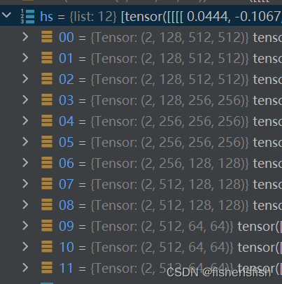
降采样之后是middle和end层,比较简单,就两层ResnetBlock,以及最后归一化然后再卷积一次输出,这样子网络设计的原因我暂不清楚,但具体而言encoder就是一系列Resnet提取图像的特征,最终的输出结果为[2,8,64,64],这里的2是由于在输入encode前对图像进行了复制处理。
        # middle
        self.mid = nn.Module()
        self.mid.block_1 = ResnetBlock(in_channels=block_in,
                                       out_channels=block_in,
                                       temb_channels=self.temb_ch,
                                       dropout=dropout)
        self.mid.attn_1 = make_attn(block_in, attn_type=attn_type)
        self.mid.block_2 = ResnetBlock(in_channels=block_in,
                                       out_channels=block_in,
                                       temb_channels=self.temb_ch,
                                       dropout=dropout)

        # end
        self.norm_out = Normalize(block_in)
        self.conv_out = torch.nn.Conv2d(block_in,
                                        2*z_channels if double_z else z_channels,
                                        kernel_size=3,
                                        stride=1,
                                        padding=1)
这里有一个求高斯分布的函数DiagonalGaussianDistribution
class DiagonalGaussianDistribution(object):
    def __init__(self, parameters, deterministic=False):
        self.parameters = parameters
        self.mean, self.logvar = torch.chunk(parameters, 2, dim=1)//沿着通道维度将输入拆分为两份,得到mean[2,4,64,64],logvar[2,4,64,64],这里的2是输入原图及其复制得到的
        self.logvar = torch.clamp(self.logvar, -30.0, 20.0)//将输入input张量每个元素的范围限制到区间 [min,max],返回结果到一个新张量。具体而言比-30小的就是-30,比20大的就是20
        self.deterministic = deterministic//默认是false,这个单词的意思叫做确定性
        self.std = torch.exp(0.5 * self.logvar)//计算标准差
        self.var = torch.exp(self.logvar)//计算方差
        if self.deterministic:
            self.var = self.std = torch.zeros_like(self.mean).to(device=self.parameters.device)

    def sample(self):
        x = self.mean + self.std * torch.randn(self.mean.shape).to(device=self.parameters.device)
        return x

    def kl(self, other=None):
        if self.deterministic:
            return torch.Tensor([0.])
        else:
            if other is None:
                return 0.5 * torch.sum(torch.pow(self.mean, 2)
                                       + self.var - 1.0 - self.logvar,
                                       dim=[1, 2, 3])
            else:
                return 0.5 * torch.sum(
                    torch.pow(self.mean - other.mean, 2) / other.var
                    + self.var / other.var - 1.0 - self.logvar + other.logvar,
                    dim=[1, 2, 3])

    def nll(self, sample, dims=[1,2,3]):
        if self.deterministic:
            return torch.Tensor([0.])
        logtwopi = np.log(2.0 * np.pi)
        return 0.5 * torch.sum(
            logtwopi + self.logvar + torch.pow(sample - self.mean, 2) / self.var,
            dim=dims)

    def mode(self):
        return self.mean
高斯分布返回的结果,这地方感觉有点玄学...为啥chunk之后就是mean,还是这只是一个命名?然后为啥图像经过encode多个resnet卷积之后就是高斯分布? 后续有解释了会更新

在SD的ddpm中,程序首先调用encode_first_stage也就是AEKL中的encode获得卷积之后的高斯分布,然后在get_first_stage_encoding中对高斯分布进行sample操作,所以最终的结果变为[2,4,64,64],也就是最终返回的隐式表达
init_latent = model.get_first_stage_encoding(model.encode_first_stage(init_image)) # move to latent space @torch.no_grad()
def encode_first_stage(self, x):
return self.first_stage_model.encode(x) def get_first_stage_encoding(self, encoder_posterior):
if isinstance(encoder_posterior, DiagonalGaussianDistribution):
z = encoder_posterior.sample()
elif isinstance(encoder_posterior, torch.Tensor):
z = encoder_posterior
else:
raise NotImplementedError(f"encoder_posterior of type '{type(encoder_posterior)}' not yet implemented")
return self.scale_factor * z def sample(self):
x = self.mean + self.std * torch.randn(self.mean.shape).to(device=self.parameters.device)
return x图像进入隐式空间后,根据珍妮大佬的图下一步应当是采样阶段?因为我并没有选择训练,但是如果是这样输入图像的目的是什么?SD确实是文本生成图像的框架,但是这个输入图像让我有点懵逼,而且还有img2img的脚本

DDPM (Denoising Diffusion Probabilistic Models)算法就是diffusion的前向和逆向过程,DDIM(Denoising Diffusion Implicit Models)则是对其速度上的改进,DDPM需要迭代上千次,而DDIM几十次就能有较好的结果,那么书接Diffusion和DDPM,让我们看看DDIM做了什么改进并取得了如此好的效果。参考大佬的DDIM介绍文章
下面的内容基于科学空间苏剑林大佬的解读,感谢!
生成扩散模型漫谈(四):DDIM = 高观点DDPM - 科学空间|Scientific Spaces (kexue.fm)
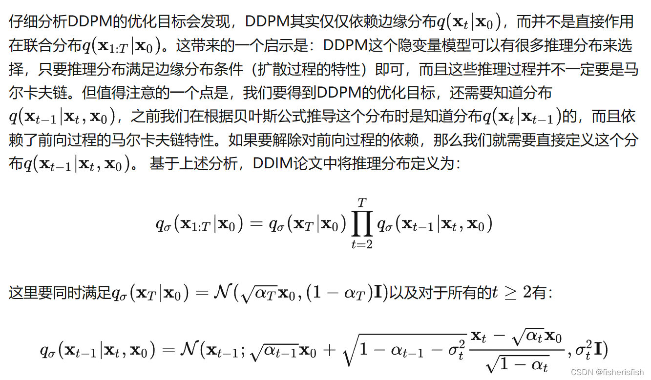
可知DDIM的核心思想就是打破马尔科夫链推导过程,重新定义每一步的推理分布,然后直接取中间步骤,从而定义一个更短的步数的前向过程,加速推导过程,也就是跳步采样的思想。
对于DDPM代码我已经在从0开始搞懂Diffusion扩散模型_fisherisfish的博客-CSDN博客文章中详细的介绍了,所以我们直接来看DDIM,当我第一次看DDIM代码的时候,我非常疑惑,因为DDIM代码里没有前向阶段,只有逆向阶段!再未完全了解DDIM的情况下,我做出了两种猜测1、DDIM沿用了DDPM的训练过程,2、DDIM不需要训练过程。在这里我个人是倾向于猜测1的,我们接着学习。
对于DDIM的整个过程,我们再一次回顾DDPM,DDPM的整体流程可以用下面式子来简化,
注意式中前向阶段的p应当是q,其中 是人为设定的高斯分布

前向阶段的损失函数如下

我们可以看出对于训练过程,
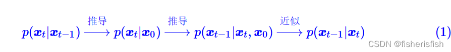
而在此过程中,有一个问题就是推导采样阶段的贝叶斯公式时,

是依赖于 ,如果我们不知道此过程,可否解出
![]()
概率论中的知识表示这其实是可以的
而且根据之前的结论,因为前向过程是正太分布,所以反向过程也应该是正太分布,
结论2:如果 q(Xt|X(t−1)) 满足高斯分布且方差β足够小,则q(X(t−1)|Xt)仍然是一个高斯分布。
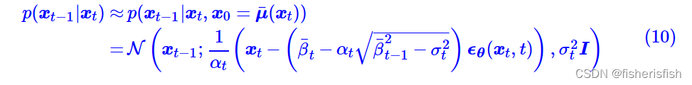
所以我们一般性地假设其为如下一个正太分布

我们为了不重新训练DDPM的前向阶段,所以保持DDPM的基础来求解这一过程
 可得到以下两个方程,即满足以下两个方程,就可以用
 直接推导
直接推导![]() 并进一步得到采样阶段的计算公式
并进一步得到采样阶段的计算公式

求解可得以下结果,注意我们在假设公式4的时候,设定了三个未知量,而我们只有两个方程,所以求解时将当做已知量,表达另外两个式子,解如下

代入式4可得,再次注意在DDPM中 是人为设定的一组极小的线性值,其中DDPM设定
=0,从1开始定义为是由0.0001 到0.02线性插值(插值数由T决定),在DDPM中
,
,故在这个式子中仅有
仍是未知的,
请注意:苏佬文章定义的是分布的标准差,而原论文中定义的
是方差,需要注意这一点差别,且苏佬文章中的
也是DDPM中的开平方值,苏佬文章中还有一个
,并不是值
的累乘,而是
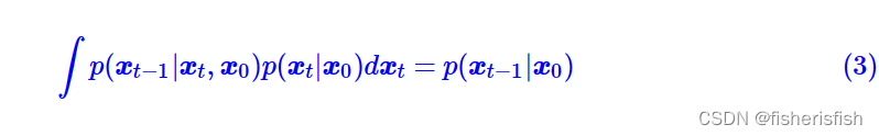
 总结:现在我们在只给定p(xt|x0)、p(xt−1|x0)的情况下,通过待定系数法求解了p(xt−1|xt,x0)的一簇解,它带有一个自由参数σt。
我们的最终目标是得到采样公式 ,所以我们需要计算X0,来去除
![]() 中的X0
中的X0
回顾DDPM的我们可以知道X0计算公式如下,注意这里论文中的等同于蓝色公式(苏佬文章)中的
,原因是苏佬定义的
是分布的标准差,而原论文中定义的
是方差,需要注意这一点差别

在苏佬的文章中,用下式来表达X0,式中的噪声项,是由Xt和t作为输入,由Unet估计出的噪声项

将式9作为X0,代入 式7就可得
式中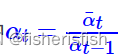 ,到了这一步我们会发现只需要通过定义
就实现了从Xt到X(t-1)的计算,这里和DDPM的公式做比较,
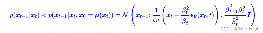
我们会发现当取 ,DDIM的推导公式就是DDPM的,注意此处的理解是DDPM是DDIM的一个特殊情况!
当我们将取0时,从Xt到X(t-1)就变成了一个固定的计算公式

总结:这也是DDIM论文中特别关心的一个例子,准确来说,原论文的DDIM就是特指σt=0的情形,其中“I”的含义就是“Implicit”,意思这是一个隐式的概率模型,因为跟其他选择所不同的是,此时从给定的xT=z出发,得到的生成结果x0是不带随机性的。后面我们将会看到,这在理论上和实用上都带来了一些好处。
那么回归到核心问题,DDIM如何加速采样过程?核心在于跳步,这里提出一个观点就是
DDPM的训练结果实质上包含了它的任意子序列参数的训练结果。
具体来说,我们训练了从[0,1,2...,T]的DDPM,那么[0~T]中的任意子序列参数的步骤也被训练了,这很好理解。
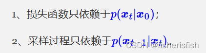
这里笔者后续又进一步加深了理解,主要是基于之前的计算公式,DDPM公式的推导是基于这个过程的,而DDIM的公式推导的目的就是排除这个过程,仅基于来计算![]() ,也就是说DDPM的公式是没办法跳步的,因为每一项的计算都依赖于相邻项的分布关系,但是DDIM通过忽视,直接从入手,而是基于人为假设的高斯分布,基于此实现的逆向公式就是可以跳步的,它并不依赖于相邻值的分布,只依赖于对于X0的分布,而对于X0的分布是已知的,所以我们就可以通过跳步来计算DDIM的采样公式!
,也就是说DDPM的公式是没办法跳步的,因为每一项的计算都依赖于相邻项的分布关系,但是DDIM通过忽视,直接从入手,而是基于人为假设的高斯分布,基于此实现的逆向公式就是可以跳步的,它并不依赖于相邻值的分布,只依赖于对于X0的分布,而对于X0的分布是已知的,所以我们就可以通过跳步来计算DDIM的采样公式!
那么当我们有一个已经训练好的T步的DDPM,我们从中取子序列来做采样阶段就可以了,假设该子序列有dim()步,那么其参数就是α¯τ1,α¯τ2,⋯,α¯dim(τ),其采样阶段也就只有dim(
)步了
这就是加速的方法,那么问题又来了,为什么要训练一个T步长的DDPM呢?直接训练一个dim()步不就行了?这里苏佬给出了两点解释
1、训练更多步数的模型也许能增强泛化能力;2、通过子序列进行加速只是其中一种加速手段,训练更充分的T步允许我们尝试更多的其他加速手段,但并不会显著增加训练成本。
到这一步,我们先解答一下之前的问题,DDIM只是一种用于采样阶段的加速方法,其加速的思想是跳步,这里笔者心中遗留了一个问题就是子序列到底是怎么取的?还有自由变量的具体作用?所以我们进入SD的DDIM实现,来进一步一探究竟!
以SD的img2img.py脚本为例,在模型创建以后,就设定为DDIMSampler,前文中,我们介绍了SD的编码部分,但值得一提的是我们使用SD时,仅使用了采样阶段,所以我们其实没有训练时的编码,我们更多是对输入图像和文字进行编码,输入图像首先通过AEKL编码进入隐式表达,然后作为X0用前向公式计算出Xt,基于此Xt,再对文字用Clip进行编码,作为条件输入并入Unet的生成噪音阶段,通过噪音不断逆向计算出另一个X0,此X0同时基于文字和图像两个条件生成,这是SDimg2img的原理,而对于txt2img,Xt则是随机生成的高斯噪声,其余步骤则是类似的。
    sampler = DDIMSampler(model)


class DDIMSampler(object):
    def __init__(self, model, schedule="linear", device=torch.device("cuda"), **kwargs):
        super().__init__()
        self.model = model
        self.ddpm_num_timesteps = model.num_timesteps
        self.schedule = schedule
        self.device = device
我们接着看SD的运行过程,在img2img中,首先对图像进行了编码,然后初始化采样器
    init_latent = model.get_first_stage_encoding(model.encode_first_stage(init_image))  # move to latent space

    sampler.make_schedule(ddim_num_steps=opt.ddim_steps, ddim_eta=opt.ddim_eta, verbose=False)
在make_schedule(附表)中,就是和DDPM中一样的初始化各种参数的过程,我们先来看一下ddim_timesteps,也就是采样的时间步t,根据之前的分析这肯定是和DDPM是不一样的,在 DDPM中直接就是设定时间步是1000,然后基于此去初始化β,而在 DDIM中,默认的取步方法是uniform(均匀),简单来说,设定ddim的timesteps数,默认是50,则相比DDPM少了20倍,加速效果也是理所应当的,所以DDIM的timesteps就是[0,20,40,...,960,980],值得注意的是这里对每一步都+1,所以最后结果是[1,21,41,...,961,981],作者给出的原因是
to get the final alpha values right (the ones from first scale to data during sampling)
    def make_schedule(self, ddim_num_steps, ddim_discretize="uniform", ddim_eta=0., verbose=True):
        self.ddim_timesteps = make_ddim_timesteps(ddim_discr_method=ddim_discretize, num_ddim_timesteps=ddim_num_steps,
                                                  num_ddpm_timesteps=self.ddpm_num_timesteps,verbose=verbose)

def make_ddim_timesteps(ddim_discr_method, num_ddim_timesteps, num_ddpm_timesteps, verbose=True):
    if ddim_discr_method == 'uniform':
        c = num_ddpm_timesteps // num_ddim_timesteps
        ddim_timesteps = np.asarray(list(range(0, num_ddpm_timesteps, c)))
    elif ddim_discr_method == 'quad':
        ddim_timesteps = ((np.linspace(0, np.sqrt(num_ddpm_timesteps * .8), num_ddim_timesteps)) ** 2).astype(int)
    else:
        raise NotImplementedError(f'There is no ddim discretization method called "{ddim_discr_method}"')

    # assert ddim_timesteps.shape[0] == num_ddim_timesteps
    # add one to get the final alpha values right (the ones from first scale to data during sampling)
    steps_out = ddim_timesteps + 1
    if verbose:
        print(f'Selected timesteps for ddim sampler: {steps_out}')
return steps_out 接着是初始化和β值,让我比较疑惑的是这里输入的
和β是从SD的v1.4.ckpt读入的,而其值并不是线性分布的,而且
值似乎也不是正常的1-β来的线性分布值累乘来的[0.9991, 0.9983, 0.9974,...,0.0047],0.9991=1*(1-0.0009),0.9983!=0.9991*(0.9991-0.0009),所以SD的v1.4版本应该不是通过线性插值来获取这两个值,或者说β不是,而
是计算误差?毕竟公式应该不会错。
        alphas_cumprod = self.model.alphas_cumprod
        assert alphas_cumprod.shape[0] == self.ddpm_num_timesteps, 'alphas have to be defined for each timestep'
        to_torch = lambda x: x.clone().detach().to(torch.float32).to(self.model.device)

        self.register_buffer('betas', to_torch(self.model.betas))
        self.register_buffer('alphas_cumprod', to_torch(alphas_cumprod))
self.register_buffer('alphas_cumprod_prev', to_torch(self.model.alphas_cumprod_prev))这一部分是前向计算和ddpm中一模一样从上到下分别是,
,
,
,
        # calculations for diffusion q(x_t | x_{t-1}) and others
        self.register_buffer('sqrt_alphas_cumprod', to_torch(np.sqrt(alphas_cumprod.cpu())))
        self.register_buffer('sqrt_one_minus_alphas_cumprod', to_torch(np.sqrt(1. - alphas_cumprod.cpu())))
        self.register_buffer('log_one_minus_alphas_cumprod', to_torch(np.log(1. - alphas_cumprod.cpu())))
        self.register_buffer('sqrt_recip_alphas_cumprod', to_torch(np.sqrt(1. / alphas_cumprod.cpu())))
        self.register_buffer('sqrt_recipm1_alphas_cumprod', to_torch(np.sqrt(1. / alphas_cumprod.cpu() - 1)))
采样阶段的值则出现了明显的不同, make_ddim_sampling_parameters输入是,ddim的采样步数,eta默认是0。我们可以看到在此函数中,首先根据ddim_timesteps对
取值,即取下标为[1,21,41,...,961,981]的这些值,此处+1的效果就显现了,+1之后可以再往前取出相应的alphas_prev值了,保证了计算链的平衡。
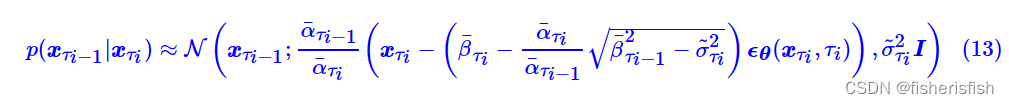
ddim这里有一个计算sigmas的公式,和DDPM中似乎有一些出入,原因是在DDIM的论文里,α符号指代的是DDPM中的,这里从代码中也能看出,输入的是alphacums即α的累乘值,此处的sigma计算公式如下
![]()
和前文的符号不同外,本质是一样的,这里再回顾一下sigma是p(X(t-1)|Xt)的标准差,如果取上式的值则和DDPM中的p(X(t-1)|Xt,X0)是一样的,在DDIM中给sigma加了一个系数值eta,当eta取1时,即DDPM,而DDIM给eta取0,此时的p(X(t-1)|Xt)是一个固定的式子
所以返回后的 ddim_alphas, ddim_alphas_prev实际上应该是ddim_alphas_cum, ddim_alphas_prev_cum
        # ddim sampling parameters
        ddim_sigmas, ddim_alphas, ddim_alphas_prev = make_ddim_sampling_parameters(alphacums=alphas_cumprod.cpu(),
                                                                                   ddim_timesteps=self.ddim_timesteps,
                                                                                   eta=ddim_eta,verbose=verbose)

def make_ddim_sampling_parameters(alphacums, ddim_timesteps, eta, verbose=True):
    # select alphas for computing the variance schedule
    alphas = alphacums[ddim_timesteps]
    alphas_prev = np.asarray([alphacums[0]] + alphacums[ddim_timesteps[:-1]].tolist())

    # according the the formula provided in https://arxiv.org/abs/2010.02502
    sigmas = eta * np.sqrt((1 - alphas_prev) / (1 - alphas) * (1 - alphas / alphas_prev))
    if verbose:
        print(f'Selected alphas for ddim sampler: a_t: {alphas}; a_(t-1): {alphas_prev}')
        print(f'For the chosen value of eta, which is {eta}, '
              f'this results in the following sigma_t schedule for ddim sampler {sigmas}')
    return sigmas, alphas, alphas_prev
继续初始化参数值, ddim_sqrt_one_minus_alphas实际上就是,值得一提的是这里还计算了DDPM的sigma值,计算公式和ddim一致,也乘了eta,也就是0,具体作用后续再看
        self.register_buffer('ddim_sigmas', ddim_sigmas)
        self.register_buffer('ddim_alphas', ddim_alphas)
        self.register_buffer('ddim_alphas_prev', ddim_alphas_prev)
        self.register_buffer('ddim_sqrt_one_minus_alphas', np.sqrt(1. - ddim_alphas))
        sigmas_for_original_sampling_steps = ddim_eta * torch.sqrt(
            (1 - self.alphas_cumprod_prev) / (1 - self.alphas_cumprod) * (
                        1 - self.alphas_cumprod / self.alphas_cumprod_prev))
        self.register_buffer('ddim_sigmas_for_original_num_steps', sigmas_for_original_sampling_steps)
初始化参数值之后, 是对输入的随机编码,输入为输入图像编码后的隐式表达init_latent,还有取样的时间步t_enc=40
t_enc = int(opt.strength * opt.ddim_steps)
# encode (scaled latent)
z_enc = sampler.stochastic_encode(init_latent, torch.tensor([t_enc] * batch_size).to(device))
我们通过回顾DDPM的公式,可知此处是通过X0,以及模型中的α值来初始化X40的值,而X40就是逆向阶段的起始高斯噪音图。
    @torch.no_grad()
    def stochastic_encode(self, x0, t, use_original_steps=False, noise=None):
        # fast, but does not allow for exact reconstruction
        # t serves as an index to gather the correct alphas
        if use_original_steps:
            sqrt_alphas_cumprod = self.sqrt_alphas_cumprod
            sqrt_one_minus_alphas_cumprod = self.sqrt_one_minus_alphas_cumprod
        else:
            sqrt_alphas_cumprod = torch.sqrt(self.ddim_alphas)
            sqrt_one_minus_alphas_cumprod = self.ddim_sqrt_one_minus_alphas

        if noise is None:
            noise = torch.randn_like(x0)

        return (extract_into_tensor(sqrt_alphas_cumprod, t, x0.shape) * x0 +
                extract_into_tensor(sqrt_one_minus_alphas_cumprod, t, x0.shape) * noise)
在采样阶段(逆向阶段)输入就是X40(z_enc),prompt编码后的特征值(c),时间步t_enc,后续的unconditional_guidance_scale和unconditional_conditioning涉及到基础知识classifier-free guidance
# decode it
samples = sampler.decode(z_enc, c, t_enc, unconditional_guidance_scale=opt.scale,
                                                 unconditional_conditioning=uc, )
先从Classifier Guidance介绍,来自于论文Diffusion Models Beat GANs on Image Synthesis,主要作用是使得扩散模型能够按类生成,具体而言就是借用别人训练好的扩散模型,我们自己再训练一个分类器,通过分类器来指定扩散模型的扩散过程。推荐苏佬的讲解,后文是本人的粗鄙理解,请见笑
生成扩散模型漫谈(九):条件控制生成结果 - 科学空间|Scientific Spaces (kexue.fm)
在DDPM的基础之上,增加条件y,那么逆向公式修正为
要计算这个式子,我们一步步来看,首先是P(X(t-1)|y)
我们用一次简单的贝叶斯公式,这个式子对于概率论新手也是友好的,hhh
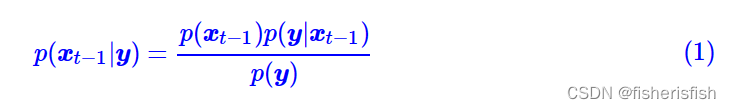
接着对每一项,都补上条件Xt,这比直接对 贝叶斯公式友好太多了,感谢苏佬的讲解。

注意,在前向过程中,xt是由x(t−1)加噪声得到的,噪声不会对分类有帮助,所以xt的加入对分类不会有任何收益,因此有p(y|x(t−1),xt)=p(y|x(t−1)),从而
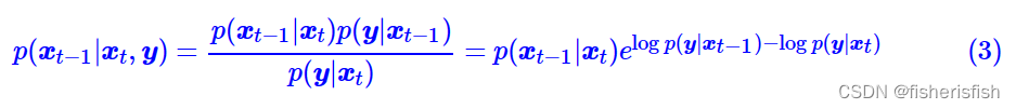
接着对右指数进行一次泰勒展开,这个地方泰勒展开就不详细讲了

在DDPM中,我们假设逆向过程也是高斯分布如下:
![]()
那么加上y以后的表达式结合式3、4如下
以此为结果,我们可以得到结论
![]()
那么我们就可以得到X(t-1)的计算公式,新增项如下
此处和原论文略有差别,差别如下
然后是经典的引入参数来调节条件参数的影响大小
 当γ>1时,生成过程将使用更多的分类器信号,结果将会提高生成结果与输入信号γ的相关性,但是会相应地降低生成结果的多样性;反之,则会降低生成结果与输入信号之间的相关性,但增加了多样性。
《More Control for Free! Image Synthesis with Semantic Diffusion Guidance》论文对γ进行了更多的解释,后续有机会进一步学习,但对于SD我们理解到这一步应该是够了
对于Classifier-Free方案,来自于论文《Classifier-Free Diffusion Guidance》,它的思想是直接将条件作为模型输入之一,用来生成噪音
![]()
训练的损失函数就是

从DDPM一路学过来就会发现这些公式本质上就是加了y作为模型输入,
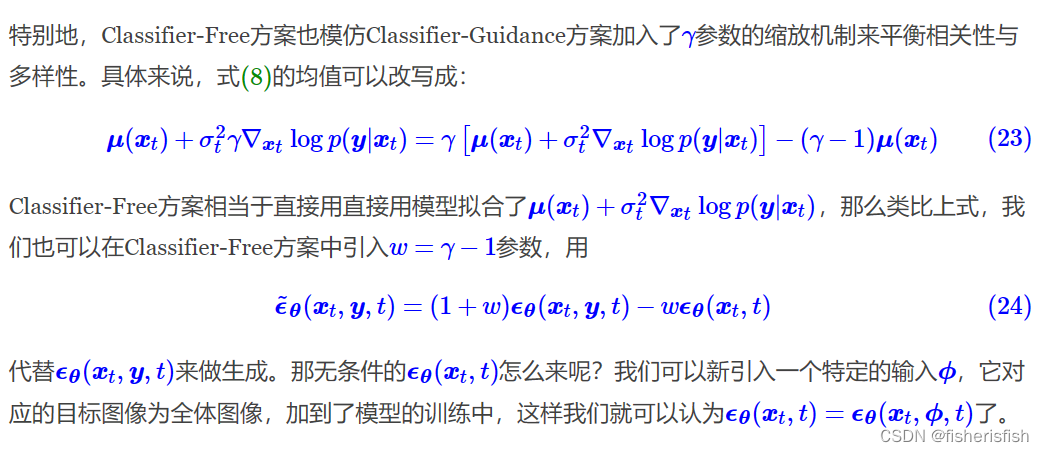 后续这部分缩放机制属于是作者个人的创新想法了,最后会浓缩为一个公式
式中α就是公式(24)中的 ,那么理解上来说,可以把c当作正向的prompt,
作为反向的prompt(negative prompt),也就是unconditional_conditioning,unconditional_guidance_scale就是α的大小
我们再回到代码部分,初版的SD,uc并非是通过人为输入的negative prompt,而是直接生成的
uc = None
if opt.scale != 1.0:
     uc = model.get_learned_conditioning(batch_size * [""])
if isinstance(prompts, tuple):
     prompts = list(prompts)
c = model.get_learned_conditioning(prompts)

# decode it
samples = sampler.decode(z_enc, c, t_enc, unconditional_guidance_scale=opt.scale,
                                                 unconditional_conditioning=uc, )
decode函数相对比较简单,循环调用p_sample_ddim,
    @torch.no_grad()
    def decode(self, x_latent, cond, t_start, unconditional_guidance_scale=1.0, unconditional_conditioning=None,
               use_original_steps=False, callback=None):

        timesteps = np.arange(self.ddpm_num_timesteps) if use_original_steps else self.ddim_timesteps
        timesteps = timesteps[:t_start]

        time_range = np.flip(timesteps)
        total_steps = timesteps.shape[0]
        print(f"Running DDIM Sampling with {total_steps} timesteps")

        iterator = tqdm(time_range, desc='Decoding image', total=total_steps)
        x_dec = x_latent
        for i, step in enumerate(iterator):
            index = total_steps - i - 1
            ts = torch.full((x_latent.shape[0],), step, device=x_latent.device, dtype=torch.long)
            x_dec, _ = self.p_sample_ddim(x_dec, cond, ts, index=index, use_original_steps=use_original_steps,
                                          unconditional_guidance_scale=unconditional_guidance_scale,
                                          unconditional_conditioning=unconditional_conditioning)
            if callback: callback(i)
        return x_dec
p_sample_ddim的代码看起来复杂,我们一段段来看,首先是前半部分由于SD是有uc输入的,所以第一个if运行else的内容,else里首先将输入的x40,和时间步t乘以2,这里讲一下t和index的区别,index实际上是DDIM的标签,比如第一次循环是从X40,生成X39,那么index值就是39,而t是原始DDPM的时间步,此时值是781,而我们的模型是DDPM训练的,所以当输入Unet计算噪音的时候,需要这个t值。乘以2的原因是需要将c和uc相结合,所以输入的X和T也乘2,来保证一致性。x_in大小[4,4,64,64],t_in大小[4,],c_in大小[4,77,768]
    @torch.no_grad()
    def p_sample_ddim(self, x, c, t, index, repeat_noise=False, use_original_steps=False, quantize_denoised=False,
                      temperature=1., noise_dropout=0., score_corrector=None, corrector_kwargs=None,
                      unconditional_guidance_scale=1., unconditional_conditioning=None,
                      dynamic_threshold=None):
        b, *_, device = *x.shape, x.device

        if unconditional_conditioning is None or unconditional_guidance_scale == 1.:
            model_output = self.model.apply_model(x, t, c)
        else:
            x_in = torch.cat([x] * 2)
            t_in = torch.cat([t] * 2)
            if isinstance(c, dict):
                assert isinstance(unconditional_conditioning, dict)
                c_in = dict()
                for k in c:
                    if isinstance(c[k], list):
                        c_in[k] = [torch.cat([
                            unconditional_conditioning[k][i],
                            c[k][i]]) for i in range(len(c[k]))]
                    else:
                        c_in[k] = torch.cat([
                                unconditional_conditioning[k],
                                c[k]])
            elif isinstance(c, list):
                c_in = list()
                assert isinstance(unconditional_conditioning, list)
                for i in range(len(c)):
                    c_in.append(torch.cat([unconditional_conditioning[i], c[i]]))
            else:
                c_in = torch.cat([unconditional_conditioning, c])
借着就是作为输入预估噪声的步骤
model_uncond, model_t = self.model.apply_model(x_in, t_in, c_in).chunk(2)
model_output = model_uncond + unconditional_guidance_scale * (model_t - model_uncond)
apply_model函数很简单,对cond做了一个增加c_crossattn的字典,然后调用model函数
    def apply_model(self, x_noisy, t, cond, return_ids=False):
        if isinstance(cond, dict):
            # hybrid case, cond is expected to be a dict
            pass
        else:
            if not isinstance(cond, list):
                cond = [cond]
            key = 'c_concat' if self.model.conditioning_key == 'concat' else 'c_crossattn'
            cond = {key: cond}

        x_recon = self.model(x_noisy, t, **cond)

        if isinstance(x_recon, tuple) and not return_ids:
            return x_recon[0]
        else:
            return x_recon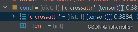
调用模型是DDPM中的DiffusionWrapper,forward代码如下,由于选择了c_crossattn所以核心代码就是elif self.conditioning_key == 'crossattn':那几行,具体而言就是cc = torch.cat(c_crossattn, 1)这一步把c_crossattn的dict又变成了cc这个tensor,大小和值均不变,是[4,77,768],然后就是输入进 out = self.diffusion_model(x, t, context=cc)
class DiffusionWrapper(pl.LightningModule):
    def __init__(self, diff_model_config, conditioning_key):
        super().__init__()
        self.sequential_cross_attn = diff_model_config.pop("sequential_crossattn", False)
        self.diffusion_model = instantiate_from_config(diff_model_config)
        self.conditioning_key = conditioning_key
        assert self.conditioning_key in [None, 'concat', 'crossattn', 'hybrid', 'adm', 'hybrid-adm', 'crossattn-adm']

    def forward(self, x, t, c_concat: list = None, c_crossattn: list = None, c_adm=None):
        if self.conditioning_key is None:
            out = self.diffusion_model(x, t)
        elif self.conditioning_key == 'concat':
            xc = torch.cat([x] + c_concat, dim=1)
            out = self.diffusion_model(xc, t)
        elif self.conditioning_key == 'crossattn':
            if not self.sequential_cross_attn:
                cc = torch.cat(c_crossattn, 1)
            else:
                cc = c_crossattn
            if hasattr(self, "scripted_diffusion_model"):
                # TorchScript changes names of the arguments
                # with argument cc defined as context=cc scripted model will produce
                # an error: RuntimeError: forward() is missing value for argument 'argument_3'.
                out = self.scripted_diffusion_model(x, t, cc)
            else:
                out = self.diffusion_model(x, t, context=cc)
        elif self.conditioning_key == 'hybrid':
            xc = torch.cat([x] + c_concat, dim=1)
            cc = torch.cat(c_crossattn, 1)
            out = self.diffusion_model(xc, t, context=cc)
        elif self.conditioning_key == 'hybrid-adm':
            assert c_adm is not None
            xc = torch.cat([x] + c_concat, dim=1)
            cc = torch.cat(c_crossattn, 1)
            out = self.diffusion_model(xc, t, context=cc, y=c_adm)
        elif self.conditioning_key == 'crossattn-adm':
            assert c_adm is not None
            cc = torch.cat(c_crossattn, 1)
            out = self.diffusion_model(x, t, context=cc, y=c_adm)
        elif self.conditioning_key == 'adm':
            cc = c_crossattn[0]
            out = self.diffusion_model(x, t, y=cc)
        else:
            raise NotImplementedError()

        return out
这里的diffusionmodel值得是modules/diffusionmodules/openaimodel.py文件中的class UNetModel(nn.Module),我们先看forwrad过程,作者注释了各个输入的含义,由于我们采用的Classifier-Free方案所以y是None
def forward(self, x, timesteps=None, context=None, y=None,**kwargs):
"""
Apply the model to an input batch.
:param x: an [N x C x ...] Tensor of inputs.
:param timesteps: a 1-D batch of timesteps.
:param context: conditioning plugged in via crossattn
:param y: an [N] Tensor of labels, if class-conditional.
:return: an [N x C x ...] Tensor of outputs.
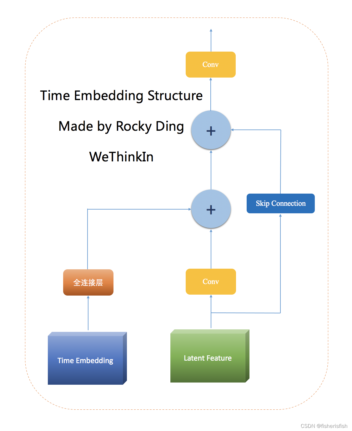
"""这里的timestep_embedding函数里出现了model_channels参数,该参数由Unet的config文件给出,在SD中一直是320, timestep_embedding的具体作用是对timesteps编码,最后结果是embedding[4,320],其中每一行值都是一样的,编码方式是sinusoidal timestep embeddings,即三角函数编码,具体计算过程看代码就明白了,编码完以后还有time_embed也就是两个线性层中间一个激活层,也就是一层MLP,激活函数是SiLU,最后的结果是[4,1280],其中1280是time_embed_dim,定义为model_channel的4倍。
Time Embedding的使用可以帮助深度学习模型更好地理解时间相关性,从而提高模型的性能。比如在Stable Diffusion中,将Time Embedding引入U-Net中,帮助其在扩散过程中从容预测噪声。
Stable Diffusion需要迭代多次对噪音进行逐步预测,使用Time Embedding就可以将time编码到网络中,从而在每一次迭代中让U-Net更加合适的噪声预测
图源见图中英文,图像复制过来就有水印,抱歉!深入浅出解析Stable Diffusion中U-Net的核心知识与价值 | 【算法兵器谱】 - 知乎 (zhihu.com)
        hs = []
        t_emb = timestep_embedding(timesteps, self.model_channels, repeat_only=False)
        emb = self.time_embed(t_emb)


def timestep_embedding(timesteps, dim, max_period=10000, repeat_only=False):
    """
    Create sinusoidal timestep embeddings.
    :param timesteps: a 1-D Tensor of N indices, one per batch element.
                      These may be fractional.
    :param dim: the dimension of the output.
    :param max_period: controls the minimum frequency of the embeddings.
    :return: an [N x dim] Tensor of positional embeddings.
    """
    if not repeat_only:
        half = dim // 2
        freqs = torch.exp(
            -math.log(max_period) * torch.arange(start=0, end=half, dtype=torch.float32) / half
        ).to(device=timesteps.device)
        args = timesteps[:, None].float() * freqs[None]
        embedding = torch.cat([torch.cos(args), torch.sin(args)], dim=-1)
        if dim % 2:
            embedding = torch.cat([embedding, torch.zeros_like(embedding[:, :1])], dim=-1)
    else:
        embedding = repeat(timesteps, 'b -> b d', d=dim)
    return embedding

time_embed_dim = model_channels * 4
self.time_embed = nn.Sequential(
            linear(model_channels, time_embed_dim),
            nn.SiLU(),
            linear(time_embed_dim, time_embed_dim),
        )
接下来的步骤和AEKL其实有点像,我们重点关注对于输入值的处理,这里的input_blocks我们需要详细看一下其组成
        h = x.type(self.dtype)
        for module in self.input_blocks:
            h = module(h, emb, context)
            hs.append(h)
在模型初始化中,input_blocks首先加了一个TimestepEmbedSequential,这玩意输入里有emb,emb是时间步t的编码,但是由于layer就是一个简单的conv_nd,这里的dims默认是2,就是一个conv_2d,in_channels是4,和model_channels一样由config决定,不过in_channels需要和输入的x的通道数保持一致,x是[4,4,64,64],注意是第二个通道。
        self.input_blocks = nn.ModuleList(
            [
                TimestepEmbedSequential(
                    conv_nd(dims, in_channels, model_channels, 3, padding=1)
                )
            ]
        )

class TimestepEmbedSequential(nn.Sequential, TimestepBlock):
    """
    A sequential module that passes timestep embeddings to the children that
    support it as an extra input.
    """

    def forward(self, x, emb, context=None):
        for layer in self:
            if isinstance(layer, TimestepBlock):
                x = layer(x, emb)
            elif isinstance(layer, SpatialTransformer):
                x = layer(x, context)
            else:
                x = layer(x)
        return x


def conv_nd(dims, *args, **kwargs):
    """
    Create a 1D, 2D, or 3D convolution module.
    """
    if dims == 1:
        return nn.Conv1d(*args, **kwargs)
    elif dims == 2:
        return nn.Conv2d(*args, **kwargs)
    elif dims == 3:
        return nn.Conv3d(*args, **kwargs)
    raise ValueError(f"unsupported dimensions: {dims}")
在config文件中有一个重要参数叫做
channel_mult: [ 1, 2, 4, 4 ]
其主要作用就是给input_blocks循环添加ResBlock以及其他的卷积层
还有一个参数叫做
num_res_blocks:2
也就是每层都要重复2个相同的ResBlock以及其他的卷积层
我们先看每一层的组成,首先就是一个ResBlock,这里直接贴ResBlock的组成部分,注意这里的ResBlock输入有x和emb两个,组合方式是广播加法,即h=h+emb_out,注意h卷积之后shape为[4,320,64,64],emb_out则是[4,320,1,1]
layers = [
                    ResBlock(
                        ch,
                        time_embed_dim,
                        dropout,
                        out_channels=mult * model_channels,
                        dims=dims,
                        use_checkpoint=use_checkpoint,
                        use_scale_shift_norm=use_scale_shift_norm,
                    )
                ]

    def _forward(self, x, emb):

        h = self.in_layers(x)
        emb_out = self.emb_layers(emb).type(h.dtype)
        while len(emb_out.shape) < len(h.shape):
            emb_out = emb_out[..., None]

        h = h + emb_out
        h = self.out_layers(h)
        return self.skip_connection(x) + h

 (0): ResBlock(
      (in_layers): Sequential(
        (0): GroupNorm32(32, 320, eps=1e-05, affine=True)
        (1): SiLU()
        (2): Conv2d(320, 320, kernel_size=(3, 3), stride=(1, 1), padding=(1, 1))
      )
      (h_upd): Identity()
      (x_upd): Identity()
      (emb_layers): Sequential(
        (0): SiLU()
        (1): Linear(in_features=1280, out_features=320, bias=True)
      )
      (out_layers): Sequential(
        (0): GroupNorm32(32, 320, eps=1e-05, affine=True)
        (1): SiLU()
        (2): Dropout(p=0, inplace=False)
        (3): Conv2d(320, 320, kernel_size=(3, 3), stride=(1, 1), padding=(1, 1))
      )
      (skip_connection): Identity()
    )
接着是添加 SpatialTransformer
Cross Attention是一种多头注意力机制,它可以在两个不同的输入序列之间建立关联,并且可以将其中一个输入序列的信息传递给另一个输入序列。
在计算机视觉中,Cross Attention可以用于将图像与文本之间的关联建立。例如,在图像字幕生成任务中,Cross Attention可以将图像中的区域与生成的文字之间建立关联,以便生成更准确的描述。
Stable Diffusion中使用Cross Attention模块控制文本信息和图像信息的融合交互,通俗来说,控制U-Net把噪声矩阵的某一块与文本里的特定信息相对应。注意此图仅为单个CrossAttention结构,并不是SpatialTransformer的结构。
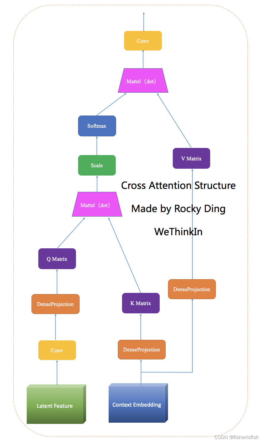
在实际操作时有两个Cross Attention,第一个CrossAttention并不会将context作为输入,而是对X做自注意力,也就是普通的SA,第二个Cross Attention才加入context,其结构和上图一致,两个attn串联后再经过feedforward层
if not exists(num_attention_blocks) or nr < num_attention_blocks[level]:
   layers.append(
         AttentionBlock(
                                ch,
                                use_checkpoint=use_checkpoint,
                                num_heads=num_heads,
                                num_head_channels=dim_head,
                                use_new_attention_order=use_new_attention_order,
                            ) if not use_spatial_transformer else SpatialTransformer(
                                ch, num_heads, dim_head, depth=transformer_depth, context_dim=context_dim,
                                disable_self_attn=disabled_sa, use_linear=use_linear_in_transformer,
                                use_checkpoint=use_checkpoint
                            )
                        )
//CrossAttention代码
class CrossAttention(nn.Module):
    def __init__(self, query_dim, context_dim=None, heads=8, dim_head=64, dropout=0.):
        super().__init__()
        inner_dim = dim_head * heads
        context_dim = default(context_dim, query_dim)

        self.scale = dim_head ** -0.5
        self.heads = heads

        self.to_q = nn.Linear(query_dim, inner_dim, bias=False)
        self.to_k = nn.Linear(context_dim, inner_dim, bias=False)
        self.to_v = nn.Linear(context_dim, inner_dim, bias=False)

        self.to_out = nn.Sequential(
            nn.Linear(inner_dim, query_dim),
            nn.Dropout(dropout)
        )

    def forward(self, x, context=None, mask=None):
        h = self.heads

        q = self.to_q(x)
        context = default(context, x)
        k = self.to_k(context)
        v = self.to_v(context)

        q, k, v = map(lambda t: rearrange(t, 'b n (h d) -> (b h) n d', h=h), (q, k, v))

        # force cast to fp32 to avoid overflowing
        if _ATTN_PRECISION =="fp32":
            with torch.autocast(enabled=False, device_type = 'cuda'):
                q, k = q.float(), k.float()
                sim = einsum('b i d, b j d -> b i j', q, k) * self.scale
        else:
            sim = einsum('b i d, b j d -> b i j', q, k) * self.scale

        del q, k

        if exists(mask):
            mask = rearrange(mask, 'b ... -> b (...)')
            max_neg_value = -torch.finfo(sim.dtype).max
            mask = repeat(mask, 'b j -> (b h) () j', h=h)
            sim.masked_fill_(~mask, max_neg_value)

        # attention, what we cannot get enough of
        sim = sim.softmax(dim=-1)

        out = einsum('b i j, b j d -> b i d', sim, v)
        out = rearrange(out, '(b h) n d -> b n (h d)', h=h)
        return self.to_out(out)

//2个CrossAttention组成BasicTransformerBlock
class BasicTransformerBlock(nn.Module):
    ATTENTION_MODES = {
        "softmax": CrossAttention,  # vanilla attention
        "softmax-xformers": MemoryEfficientCrossAttention
    }
    def __init__(self, dim, n_heads, d_head, dropout=0., context_dim=None, gated_ff=True, checkpoint=True,
                 disable_self_attn=False):
        super().__init__()
        attn_mode = "softmax-xformers" if XFORMERS_IS_AVAILBLE else "softmax"
        assert attn_mode in self.ATTENTION_MODES
        attn_cls = self.ATTENTION_MODES[attn_mode]
        self.disable_self_attn = disable_self_attn
        self.attn1 = attn_cls(query_dim=dim, heads=n_heads, dim_head=d_head, dropout=dropout,
                              context_dim=context_dim if self.disable_self_attn else None)  # is a self-attention if not self.disable_self_attn
        self.ff = FeedForward(dim, dropout=dropout, glu=gated_ff)
        self.attn2 = attn_cls(query_dim=dim, context_dim=context_dim,
                              heads=n_heads, dim_head=d_head, dropout=dropout)  # is self-attn if context is none
        self.norm1 = nn.LayerNorm(dim)
        self.norm2 = nn.LayerNorm(dim)
        self.norm3 = nn.LayerNorm(dim)
        self.checkpoint = checkpoint

    def forward(self, x, context=None):
        return checkpoint(self._forward, (x, context), self.parameters(), self.checkpoint)

    def _forward(self, x, context=None):
        x = self.attn1(self.norm1(x), context=context if self.disable_self_attn else None) + x
        x = self.attn2(self.norm2(x), context=context) + x
        x = self.ff(self.norm3(x)) + x
        return x

//SpatialTransformer的forward,和普通的Transformer类似,其中的block只有一个BasicTransformerBlock
    def forward(self, x, context=None):
        # note: if no context is given, cross-attention defaults to self-attention
        if not isinstance(context, list):
            context = [context]
        b, c, h, w = x.shape
        x_in = x
        x = self.norm(x)
        if not self.use_linear:
            x = self.proj_in(x)
        x = rearrange(x, 'b c h w -> b (h w) c').contiguous()
        if self.use_linear:
            x = self.proj_in(x)
        for i, block in enumerate(self.transformer_blocks):
            x = block(x, context=context[i])
        if self.use_linear:
            x = self.proj_out(x)
        x = rearrange(x, 'b (h w) c -> b c h w', h=h, w=w).contiguous()
        if not self.use_linear:
            x = self.proj_out(x)
        return x + x_in


   (1): SpatialTransformer(
      (norm): GroupNorm(32, 320, eps=1e-06, affine=True)
      (proj_in): Conv2d(320, 320, kernel_size=(1, 1), stride=(1, 1))
      (transformer_blocks): ModuleList(
        (0): BasicTransformerBlock(
          (attn1): CrossAttention(
            (to_q): Linear(in_features=320, out_features=320, bias=False)
            (to_k): Linear(in_features=320, out_features=320, bias=False)
            (to_v): Linear(in_features=320, out_features=320, bias=False)
            (to_out): Sequential(
              (0): Linear(in_features=320, out_features=320, bias=True)
              (1): Dropout(p=0.0, inplace=False)
            )
          )
          (ff): FeedForward(
            (net): Sequential(
              (0): GEGLU(
                (proj): Linear(in_features=320, out_features=2560, bias=True)
              )
              (1): Dropout(p=0.0, inplace=False)
              (2): Linear(in_features=1280, out_features=320, bias=True)
            )
          )
          (attn2): CrossAttention(
            (to_q): Linear(in_features=320, out_features=320, bias=False)
            (to_k): Linear(in_features=768, out_features=320, bias=False)
            (to_v): Linear(in_features=768, out_features=320, bias=False)
            (to_out): Sequential(
              (0): Linear(in_features=320, out_features=320, bias=True)
              (1): Dropout(p=0.0, inplace=False)
            )
          )
          (norm1): LayerNorm((320,), eps=1e-05, elementwise_affine=True)
          (norm2): LayerNorm((320,), eps=1e-05, elementwise_affine=True)
          (norm3): LayerNorm((320,), eps=1e-05, elementwise_affine=True)
        )
      )
      (proj_out): Conv2d(320, 320, kernel_size=(1, 1), stride=(1, 1))
    )
  )
我们先总结一下,此时一个ResNet后接一个SpatialTransformer,然后该组件根据num_res_blocks
需要循环两次接入模型中,其中ResNet的输入是X和emb,也就是输入图像和时间之间特征,SpatialTransformer则是在此特征上再加上了context,至此三个输入之间都建立起了联系,我们也搞明白了是如何处理的,最后就是根据Unet的结构搭建整个模型了,中间还有降采样和上采样过程
(1-2): 2 x TimestepEmbedSequential(
      (0): ResBlock(
        (in_layers): Sequential(
          (0): GroupNorm32(32, 320, eps=1e-05, affine=True)
          (1): SiLU()
          (2): Conv2d(320, 320, kernel_size=(3, 3), stride=(1, 1), padding=(1, 1))
        )
        (h_upd): Identity()
        (x_upd): Identity()
        (emb_layers): Sequential(
          (0): SiLU()
          (1): Linear(in_features=1280, out_features=320, bias=True)
        )
        (out_layers): Sequential(
          (0): GroupNorm32(32, 320, eps=1e-05, affine=True)
          (1): SiLU()
          (2): Dropout(p=0, inplace=False)
          (3): Conv2d(320, 320, kernel_size=(3, 3), stride=(1, 1), padding=(1, 1))
        )
        (skip_connection): Identity()
      )
      (1): SpatialTransformer(
        (norm): GroupNorm(32, 320, eps=1e-06, affine=True)
        (proj_in): Conv2d(320, 320, kernel_size=(1, 1), stride=(1, 1))
        (transformer_blocks): ModuleList(
          (0): BasicTransformerBlock(
            (attn1): CrossAttention(
              (to_q): Linear(in_features=320, out_features=320, bias=False)
              (to_k): Linear(in_features=320, out_features=320, bias=False)
              (to_v): Linear(in_features=320, out_features=320, bias=False)
              (to_out): Sequential(
                (0): Linear(in_features=320, out_features=320, bias=True)
                (1): Dropout(p=0.0, inplace=False)
              )
            )
            (ff): FeedForward(
              (net): Sequential(
                (0): GEGLU(
                  (proj): Linear(in_features=320, out_features=2560, bias=True)
                )
                (1): Dropout(p=0.0, inplace=False)
                (2): Linear(in_features=1280, out_features=320, bias=True)
              )
            )
            (attn2): CrossAttention(
              (to_q): Linear(in_features=320, out_features=320, bias=False)
              (to_k): Linear(in_features=768, out_features=320, bias=False)
              (to_v): Linear(in_features=768, out_features=320, bias=False)
              (to_out): Sequential(
                (0): Linear(in_features=320, out_features=320, bias=True)
                (1): Dropout(p=0.0, inplace=False)
              )
            )
            (norm1): LayerNorm((320,), eps=1e-05, elementwise_affine=True)
            (norm2): LayerNorm((320,), eps=1e-05, elementwise_affine=True)
            (norm3): LayerNorm((320,), eps=1e-05, elementwise_affine=True)
          )
        )
        (proj_out): Conv2d(320, 320, kernel_size=(1, 1), stride=(1, 1))
      )
    )
整个模型如下图
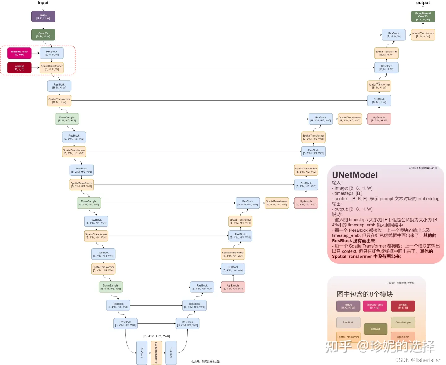
我们再回到前面调用模型的步骤,根据之前的推导Unet的输出是噪音,也就是这个x_recon
def apply_model(self, x_noisy, t, cond, return_ids=False):
if isinstance(cond, dict):
# hybrid case, cond is expected to be a dict
pass
else:
if not isinstance(cond, list):
cond = [cond]
key = 'c_concat' if self.model.conditioning_key == 'concat' else 'c_crossattn'
cond = {key: cond}
x_recon = self.model(x_noisy, t, **cond)
if isinstance(x_recon, tuple) and not return_ids:
return x_recon[0]
else:
return x_recon
注意我们之前在输入的时候,x_in是复制了两份的,所以输出后需要chunk,这里结合之前的c_in是uncond+c,所以此时前两个通道是model_uncond,是 ,后两个通道才是我们心心念念的model_t,也就是
model_output就是下面这个公式
            model_uncond, model_t = self.model.apply_model(x_in, t_in, c_in).chunk(2)
            model_output = model_uncond + unconditional_guidance_scale * (model_t - model_uncond)
再之后就是反向计算X(t-1)了,在classier-free中,计算公式是和DDPM\DDIM一致的,
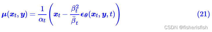
在代码中,首先计算了X0,依据公式是
然后在基于X0,计算X(t-1),依据公式和上面是一样的,但是后面的噪音部分有变化,具体而言就是重新加上了sigma_t,不过在DDIM中,sigma_t是取0的,所以还是一样的....,相当于增加一些随机性吧,这里其实有一点疑惑在于既然可以直接计算X0了,为什么还要一步步计算X(t-1),个人的猜测是直接计算X0,效果可能非常差,还有一个可能是没有随机性,生成图像和输入图像是一样的
        pred_x0 = (x - sqrt_one_minus_at * e_t) / a_t.sqrt()

 # direction pointing to x_t
        dir_xt = (1. - a_prev - sigma_t**2).sqrt() * e_t
        noise = sigma_t * noise_like(x.shape, device, repeat_noise) * temperature
        if noise_dropout > 0.:
            noise = torch.nn.functional.dropout(noise, p=noise_dropout)
        x_prev = a_prev.sqrt() * pred_x0 + dir_xt + noise
后面的这些步骤其实就简单了,有些人可能会疑惑为啥是samples而不是sample,因为最开始的输入的z_enc就是[2,4,64,64],所以最后的samples也是[2,4,64,64],解码之后就会生成两张图像,而且还是一正一反的,这个反感觉就是model_uncond给出的
# decode it
samples = sampler.decode(z_enc, c, t_enc, unconditional_guidance_scale=opt.scale,
                                                 unconditional_conditioning=uc, )
x_samples = model.decode_first_stage(samples)
x_samples = torch.clamp((x_samples + 1.0) / 2.0, min=0.0, max=1.0)

for x_sample in x_samples:
    x_sample = 255. * rearrange(x_sample.cpu().numpy(), 'c h w -> h w c')
    img = Image.fromarray(x_sample.astype(np.uint8))
    img = put_watermark(img, wm_encoder)
    img.save(os.path.join(sample_path, f"{base_count:05}.png"))
                            base_count += 1
all_samples.append(x_samples)
总结:这篇文章到这里已经4W字了,可能中间有非常多没有必要的内容,但对于一个初学者来说,想要完全搞懂SD这些内容可能都是不够的,对于我个人来说,写完以后,对于SD有了非常清晰的认识,解决了非常多的困惑,学会了很多新知识,下一篇文章将是ControlNet
在训练阶段,SD首先对输入图像进行AEKL编码,SD的AEKL编码由许多ResNet块组成进行特征提取并编码,并经过一个求高斯分布的函数DiagonalGaussianDistribution进行高斯采样,最终将输入图像[2,3,512,512],编码为[2,4,64,64],后续的训练阶段同DDPM,进行前向推导,计算KL散度损失函数,优化Unet模型,在训练过程中,同样有prompts编码的c以及时间步t作为输入。
在采样阶段,对于txt2img随机生成初始的高斯噪音图像,对于img2img,输入的img同样需要AEKL编码进隐式表达,latent_input会根据模型ckpt提供的α值和β值直接计算为X40,作为初始的高斯分布噪音从而影响到图像生成,此外采样阶段采用DDIM方法,进行跳步采样,并且改变了反向过程的计算公式,实现了加速。
SD使用的Unet模型中加入了Time Embedding,作用是编码时间步使之可以加入到Unet作为输入,时间步特征加入到了Unet的ResNet Block中;还加入了crossattention,其是self-attention的变种,可以在两个不同的输入序列之间建立关联,并且可以将其中一个输入序列的信息传递给另一个输入序列,并由crossattention构建SpatialTransformer,其输入了文本编码形成的context信息。
遗留的问题:
1、SD中AEKL和Unet结构的原因,是否是大小和性能的平衡?