0.前言:
上一篇使用sklearn库调用八个机器学习模型对DEAP情感数据进行分类,本篇我自己建立了几个CNN模型去处理,本次研究的目的包括:
1、探究个人建立cnn模型的可行性
2、模型训练90%以上,但测试ACC在60%左右原因(不是过拟合,我已多次验证不是过拟合原因)
我之前在STEW数据集上花费大量时间设计处理该数据的CNN模型,参照了相关论文的cnn设计思路,我的设计思路有两种:
1、原始EEG信号输入,cnn模型卷积层先时域后空间域(论文中此组合最多),卷积后接激活层、BN层(实验证明,BN接在激活后效果更好)、池化层、Fc1、Dropout、Fc2、Fc3。(这样设计的模型各个超参数我都考虑到了,卷积+池化的kernel_size和stride,这样做的结果是最后一层池化出来的数据,喂给Fc1的数据是4096个,4096是VGGNet第一层fc的数量)
2、DWT、PSD提取特征输入,model结构如上。
上面在STEW上的验证采用pytorch编写,我确定模型不是过拟合,也对数据做了不同的预处理工程,结果还是测试acc不行,于是我换了个数据,在DEAP上再做一下,并改用Tensorflow编写方式,之前做的都是pytorch编写。我之前忘了在哪看到过,有人把pytorch和Tensorflow进行了详细的对比,什么pytorch编写简洁方便的不多说,有趣的是我记得他提过这两种方式编写同样模型性能的出入,涉及了过拟合和最终性能问题,应该是在知乎看的,但没有收藏。
下面直接给出本次设计的模型和对应的结果,再次查看用Tensorflow建立CNN模型,数据做好预处理,还是会发生train=90%,test=60%的情况吗?
1.导入库
import pandas as pd
import tensorflow as tf
import numpy as np
import tensorflow.keras as keras
from tensorflow.keras import Sequential
from tensorflow.keras.layers import Conv1D
from tensorflow.keras.layers import MaxPooling1D
from tensorflow.keras.layers import Flatten
from tensorflow.keras.layers import Dense
from tensorflow.keras.layers import Dropout
from tensorflow.keras.layers import BatchNormalization
from tensorflow.keras.layers import Softmax
from sklearn.metrics import classification_report
from keras.utils.vis_utils import plot_model
from sklearn.preprocessing import StandardScaler
import matplotlib.pyplot as plt
import pickle
from scipy.stats import zscore
from sklearn.model_selection import train_test_split
from sklearn import preprocessing
import gc
from keras.callbacks import ReduceLROnPlateau
from collections import Counter
import seaborn as sns
from sklearn.metrics import confusion_matrix
from sklearn.utils.class_weight import compute_class_weight
from imblearn.over_sampling import RandomOverSampler, SMOTE, ADASYN
2.导入数据
all_sub_data = np.load("/content/drive/MyDrive/major project/all_sub_data.npy")
print(all_sub_data.shape)
我们可知DEAP共32位被试,32导联,每个被试1280个样本,一个通道有8064个数据。
3.数据归一化
for sub in range(all_sub_data.shape[0]):
  all_sub_data[sub] = zscore(all_sub_data[sub], axis = 1)  #zscore normalize each channel
gc.collect()all_sub_data就是我们后面要使用的数据了。我们对它做归一化处理,预处理中别的步骤可以不做,但归一化必须做,做不做归一化的数据,模型最后的精度是天差地别的。后面分的train/test也是从all_sub_data中取的。
4.标签重新编码
if(inp_choice == 'm'):
  labels = pd.read_excel("/content/drive/MyDrive/major project/metadata/Labels.xls")
  #for multiclass classification
  sub_labels = labels["Valence-Arousal Model Quadrant"].astype('int')
  gc.collect()
  sub_labels

if(inp_choice == 'm'):
  labels = pd.read_excel("/content/drive/MyDrive/major project/metadata/Labels.xls")
  #for multiclass classification
  sub_labels = labels["Valence-Arousal Model Quadrant"].astype('int')
  gc.collect()
  sub_labels

#Distribution of Multi-Class Labels
if(inp_choice == 'm'):
  #SKIP FOR BINARY CLASSIFICATION
  # Add frequency bar plot here for dataset label distribution
  c = Counter(sub_labels)
  print(c)
  plt.figure()
  plt.bar([0,1,2,3], [c[0], c[1], c[2], c[3]])
  plt.show()

#Distribution of Binary Class Labels
if(inp_choice == 'b'):
  # Add frequency bar plot here for dataset label distribution
  c = Counter(sub_labels)
  print(c)
  plt.figure()
  plt.bar([0,1], [c[0], c[1]])
  plt.show()

### Label Binarization of multi-class labels
if(inp_choice == 'm'):
  multi_class_weights = compute_class_weights("balanced", classes = [0,1,2,3], y=sub_labels)
  print(multi_class_weights)
  d_multi_class_weights = dict(enumerate(multi_class_weights))
  print(d_multi_class_weights)

if(inp_choice == 'm'):
  lb = preprocessing.LabelBinarizer()
  sub_labels = lb.fit_transform(sub_labels)
  print(lb.classes_)
  print(sub_labels.shape)
  print(sub_labels)

### Label Binarization of 2/Binary labels
if(inp_choice == 'b'):
  bin_class_weights = compute_class_weight("balanced", classes = [0,1], y=sub_labels)
  print(bin_class_weights)
  d_bin_class_weights = dict(enumerate(bin_class_weights))
  print(d_bin_class_weights)

def encode(x):
  if(x==1):
    return [0,1]
  elif(x==0):
    return [1,0]
  else:
    print("invalid value")
    return None

if(inp_choice == 'b'):
  sub_labels_bin = np.array(list(map(encode, sub_labels)))
  print(sub_labels_bin.shape)
  print(sub_labels_bin[:6])

if(inp_choice == 'b'):
  sub_labels_bin[0]

if(inp_choice == 'b'):
  sub_labels = sub_labels_bin
  gc.collect()
  print(sub_labels.shape)

def inv_bin(x):
  if(x == [0,1]):
     return 1
  elif(x==[1,0]):
    return 0
5.划分训练集、测试集
X_train, X_test, y_train, y_test = train_test_split(all_sub_data, sub_labels, test_size =
                                                   0.1, random_state = 42,shuffle = True,
                                                   stratify = sub_labels)

X_train.shape, y_train.shape, X_test.shape, y_test.shape

我这里是把1280个样本9/1分给了训练集\测试集
6.数据增强
随机选取三位被试者12、6、4,对他们使用不同大小的窗口做数据增强
#12,6 and 4 subsignals are generated from 8064 length EEG signal, labels repeated accordingly
y_train_12 = np.repeat(y_train, 12, axis = 0)
#y_train_6 = np.repeat(y_train, 6, axis = 0)
#y_train_4 = np.repeat(y_train, 4, axis = 0)
del(y_train)
gc.collect()
#print(y_train_12.shape, y_train_6.shape, y_train_4.shape)
print(y_train_12.shape)

try:
  del y_train_6, y_train_4
except:
  pass
gc.collect()

try:
  del c_train, c_test, c_train_12, c
except:
  pass
gc.collect()
## Loading Training data with different window sizes
channel_wise = np.transpose(X_train, (1,0,2))
del(X_train)
gc.collect()
def process_input(instances, sub_signals):
#instances must be channel wise of shape (32, -1, 8064)
samples = int(8064/sub_signals)
transformed = []
for i in range(instances.shape[0]):
transformed.append(np.reshape(instances[i], (-1,samples,1)))
transformed = np.array(transformed)
print(transformed.shape, 'is the shape obtained.')
gc.collect()
return transformed
### 12 sub signals of length 672 each, total 13824 instances
#X_train_12 = np.load("/content/drive/MyDrive/major project/data_augmentation/channel_wise_12.npy")
#print(X_train_12.shape, 'Shape of Training Data')
X_train_12 = process_input(channel_wise, 12)
gc.collect()
同理,sub6和sub4通过数据增强后是
#X_train_6 = np.load("/content/drive/MyDrive/major project/data_augmentation/channel_wise_6.npy")
#print(X_train_6.shape, 'Shape of Training Data')
#gc.collect()

#X_train_4 = np.load("/content/drive/MyDrive/major project/data_augmentation/channel_wise_4.npy")
#print(X_train_4.shape, 'Shape of Training Data')
#gc.collect()
7.改变数据输入形状
def process_input_ensemble(instances, sub_signals):
  """
  This Function explicity adds a dimension for the sub_signals, hence is used for ensembel modeling to traverse that dimension.
  Otherwise also we can simply assume, since the dataset is ordered that the groups of len(sub_signals) are obtained from one EEG signal
  """
  #instances must be channel wise of shape (32, -1, 8064)
  gc.collect()
  samples = int(8064/sub_signals)
  transformed = []
  for i in range(instances.shape[0]):
    transformed.append(np.reshape(instances[i], (-1,sub_signals,samples,1)))
    gc.collect()
  transformed = np.array(transformed)
  print(transformed.shape, 'is the shape obtained.')
  gc.collect()
  #output shape will be (len(intances), 32, sub_signals, samples, 1)
  return transformed

X_test_channels = np.transpose(X_test, (1,0,2))
x_test_12 = process_input(X_test_channels, 12)
y_test_12 = np.repeat(np.array(y_test), 12, axis = 0)
print(x_test_12.shape, y_test_12.shape)

"""
x_test_6 = process_input(X_test_channels, 6)
y_test_6 = np.repeat(np.array(y_test), 6, axis = 0)
print(x_test_6.shape, y_test_6.shape)
"""

"""
x_test_6 = process_input(X_test_channels, 6)
y_test_6 = np.repeat(np.array(y_test), 6, axis = 0)
print(x_test_6.shape, y_test_6.shape)
"""
8.定义混淆矩阵+loss、acc图
def plot_evaluation_curves(history, EPOCHS, mtrc):
  acc = history.history[mtrc[0]]
  val_acc = history.history[mtrc[1]]

  loss = history.history['loss']
  val_loss = history.history['val_loss']

  epochs_range = range(EPOCHS)

  plt.figure(figsize=(10, 6))
  plt.subplot(1, 2, 1)
  plt.plot(epochs_range, acc, label='Training ' + mtrc[0])
  plt.plot(epochs_range, val_acc, label='Validation '+ mtrc[0])
  plt.legend(loc='lower right')
  plt.title('Training and Validation ' +  mtrc[0])

  plt.subplot(1, 2, 2)
  plt.plot(epochs_range, loss, label='Training Loss')
  plt.plot(epochs_range, val_loss, label='Validation Loss')
  plt.legend(loc='upper right')
  plt.title('Training and Validation Loss')
  plt.show()

def make_confusion_matrix(cf,
                          group_names=None,
                          categories='auto',
                          count=True,
                          percent=True,
                          cbar=True,
                          xyticks=True,
                          xyplotlabels=True,
                          sum_stats=True,
                          figsize=None,
                          cmap='Blues',
                          title=None):
    '''
    This function will make a pretty plot of an sklearn Confusion Matrix cm using a Seaborn heatmap visualization.
    Arguments
    ---------
    cf:            confusion matrix to be passed in
    group_names:   List of strings that represent the labels row by row to be shown in each square.
    categories:    List of strings containing the categories to be displayed on the x,y axis. Default is 'auto'
    count:         If True, show the raw number in the confusion matrix. Default is True.
    normalize:     If True, show the proportions for each category. Default is True.
    cbar:          If True, show the color bar. The cbar values are based off the values in the confusion matrix.
                   Default is True.
    xyticks:       If True, show x and y ticks. Default is True.
    xyplotlabels:  If True, show 'True Label' and 'Predicted Label' on the figure. Default is True.
    sum_stats:     If True, display summary statistics below the figure. Default is True.
    figsize:       Tuple representing the figure size. Default will be the matplotlib rcParams value.
    cmap:          Colormap of the values displayed from matplotlib.pyplot.cm. Default is 'Blues'
                   See http://matplotlib.org/examples/color/colormaps_reference.html

    title:         Title for the heatmap. Default is None.
    '''


    # CODE TO GENERATE TEXT INSIDE EACH SQUARE
    blanks = ['' for i in range(cf.size)]

    if group_names and len(group_names)==cf.size:
        group_labels = ["{}\n".format(value) for value in group_names]
    else:
        group_labels = blanks

    if count:
        group_counts = ["{0:0.0f}\n".format(value) for value in cf.flatten()]
    else:
        group_counts = blanks

    if percent:
        group_percentages = ["{0:.2%}".format(value) for value in cf.flatten()/np.sum(cf)]
    else:
        group_percentages = blanks

    box_labels = [f"{v1}{v2}{v3}".strip() for v1, v2, v3 in zip(group_labels,group_counts,group_percentages)]
    box_labels = np.asarray(box_labels).reshape(cf.shape[0],cf.shape[1])


    # CODE TO GENERATE SUMMARY STATISTICS & TEXT FOR SUMMARY STATS
    if sum_stats:
        #Accuracy is sum of diagonal divided by total observations
        accuracy  = np.trace(cf) / float(np.sum(cf))

        #if it is a binary confusion matrix, show some more stats
        if len(cf)==2:
            #Metrics for Binary Confusion Matrices
            precision = cf[1,1] / sum(cf[:,1])
            recall    = cf[1,1] / sum(cf[1,:])
            f1_score  = 2*precision*recall / (precision + recall)
            stats_text = "\n\nAccuracy={:0.3f}\nPrecision={:0.3f}\nRecall={:0.3f}\nF1 Score={:0.3f}".format(
                accuracy,precision,recall,f1_score)
        else:
            stats_text = "\n\nAccuracy={:0.3f}".format(accuracy)
    else:
        stats_text = ""


    # SET FIGURE PARAMETERS ACCORDING TO OTHER ARGUMENTS
    if figsize==None:
        #Get default figure size if not set
        figsize = plt.rcParams.get('figure.figsize')

    if xyticks==False:
        #Do not show categories if xyticks is False
        categories=False


    # MAKE THE HEATMAP VISUALIZATION
    plt.figure(figsize=figsize)
    sns.heatmap(cf,annot=box_labels,fmt="",cmap=cmap,cbar=cbar,xticklabels=categories,yticklabels=categories)

    if xyplotlabels:
        plt.ylabel('True label')
        plt.xlabel('Predicted label' + stats_text)
    else:
        plt.xlabel(stats_text)

    if title:
        plt.title(title)

def show_test_metrics(x_test, y_test, model):
  print("Testing Set MEASURES: ")
  #Testing Data metrics
  pred_y = model.predict(x_test)
  c_pred = Counter(np.argmax(pred_y, axis = 1))
  print(c_pred, "Predicted Distribution of Testing Dataset")
  c_true = Counter(np.argmax(y_test, axis = 1))
  print(c_true, "Actual Distribution of Testing Dataset")
  print(model.evaluate(x_test, y_test), "Testing Measures of Model.")
  print("Classification Report of Model on Testing Data")
  print(classification_report(np.argmax(y_test, axis =1), np.argmax(model.predict(x_test), axis = 1) , digits = 4) )
  make_confusion_matrix(confusion_matrix(np.argmax(y_test, axis = 1), np.argmax(model.predict(x_test), axis = 1)))
  print("------------------------------------------------------------\n")


def show_metrics(x_train=None, x_val=None, y_train=None, y_val=None, model=None):
  print("TRAINING MEASURES: ")
  #Training Data metrics
  pred_y = model.predict(x_train)
  c_pred = Counter(np.argmax(pred_y, axis = 1))
  print(c_pred, "Predicted Distribution of Training Dataset")
  c_true = Counter(np.argmax(y_train, axis = 1))
  print(c_true, "Actual Distribution of Training Dataset")
  print(model.evaluate(x_train, y_train), "Training Measures of Model.")
  print("Classification Report of Model on Training Data")
  print(classification_report(np.argmax(y_train, axis =1), np.argmax(model.predict(x_train), axis = 1) , digits = 4) )
  make_confusion_matrix(confusion_matrix(np.argmax(y_train, axis = 1), np.argmax(model.predict(x_train), axis = 1)))
  print("\n------------------------------------------------------------------------------------------\n")

  #Validation Data Metrics
  print("VALIDATION MEASURES: ")
  pred_y = model.predict(x_val)
  c_pred = Counter(np.argmax(pred_y, axis = 1))
  print(c_pred, "Predicted Distribution of Validation Dataset")
  c_true = Counter(np.argmax(y_val, axis = 1))
  print(c_true, "Actual Distribution of Validation Dataset")
  print(model.evaluate(x_val, y_val), "Validation Measures of Model.")
  print("Classification Report of Model on Validation Data")
  print(classification_report(np.argmax(y_val, axis = 1), np.argmax(model.predict(x_val), axis = 1), digits = 4))
  make_confusion_matrix(confusion_matrix(np.argmax(y_val, axis = 1), np.argmax(model.predict(x_val), axis =1)) )
  print("\n------------------------------------------------------------------------------------------\n")
  gc.collect()
9.Tensorflow搭建CNN模型
METRICS = [
      keras.metrics.TruePositives(name='tp'),
      keras.metrics.FalsePositives(name='fp'),
      keras.metrics.TrueNegatives(name='tn'),
      keras.metrics.FalseNegatives(name='fn'),
      keras.metrics.BinaryAccuracy(name='accuracy'),
      keras.metrics.Precision(name='precision'),
      keras.metrics.Recall(name='recall'),
      keras.metrics.AUC(name='auc'),
]

def dummy_models(sub_signals=12, metrics = METRICS):
  sample_size = int(8064/sub_signals)
  models = [0]*32
  for i in range(32):
    models[i] = Sequential()
    models[i].add(Dense(100, activation = 'relu', input_shape = (sample_size, 1)))
    models[i].add(Flatten())
    models[i].add(Dense(40, activation = 'relu'))
    try:
      #fc2 and softmax
      if (inp_choice == 'b'):
        #binary classification
        models[i].add(Dense(2,  activation = 'softmax'))
        models[i].compile(optimizer= tf.keras.optimizers.Adam(learning_rate = 1e-4) , loss = tf.keras.losses.BinaryCrossentropy(), metrics= metrics)
      elif (inp_choice == 'm'):
        #mutliclass classification
        models[i].add(Dense(4, activation = 'softmax'))
        models[i].compile(optimizer= tf.keras.optimizers.Adam(learning_rate=1e-4) , loss = tf.keras.losses.CategoricalCrossentropy(), metrics= metrics)
    except ValueError:
      raise ValueError("ValueError exception thrown. Invalid Classfication choice, No Model was Created")
  print("All models defined.")
  return models

null_data = np.zeros((13824, 672, 1))

def create_models(dense_par=20, sub_signals=12, metrics = METRICS):
  sample_size = int(8064/sub_signals)
  models = [0]*32
  for i in range(32):
    models[i] = Sequential()
    #block 1
    models[i].add(Conv1D(filters=32, kernel_size=5,strides = 3, input_shape=(sample_size, 1)))
    models[i].add(BatchNormalization())
    models[i].add(tf.keras.layers.Activation('relu'))

    #block 2
    models[i].add(Conv1D(filters=24, kernel_size=3,strides = 2))
    models[i].add(BatchNormalization())
    models[i].add(tf.keras.layers.Activation('relu'))

    #block 3
    models[i].add(Conv1D(filters=16, kernel_size=3,strides = 2))
    models[i].add(BatchNormalization())
    models[i].add(tf.keras.layers.Activation('relu'))

    #block 4
    models[i].add(Conv1D(filters=8, kernel_size=3,strides = 2))
    models[i].add(BatchNormalization())
    models[i].add(tf.keras.layers.Activation('relu'))

    #fc-1
    models[i].add(Flatten())
    models[i].add(Dense(dense_par, activation='relu'))

    #dropout
    models[i].add(Dropout(rate = 0.5))
    try:
      #fc2 and softmax
      if (inp_choice == 'b'):
        #binary classification
        models[i].add(Dense(2,  activation = 'softmax'))
        models[i].compile(optimizer= tf.keras.optimizers.Adam(learning_rate = 1e-4) , loss = tf.keras.losses.BinaryCrossentropy(), metrics= metrics)
      elif (inp_choice == 'm'):
        #mutliclass classification
        models[i].add(Dense(4, activation = 'softmax'))
        models[i].compile(optimizer= tf.keras.optimizers.Adam(learning_rate=1e-4) , loss = tf.keras.losses.CategoricalCrossentropy(), metrics= metrics)
    except ValueError:
      raise ValueError("ValueError exception thrown. Invalid Classfication choice, No Model was Created")
  print("All models defined.")
  return models
10.cnn训练测试
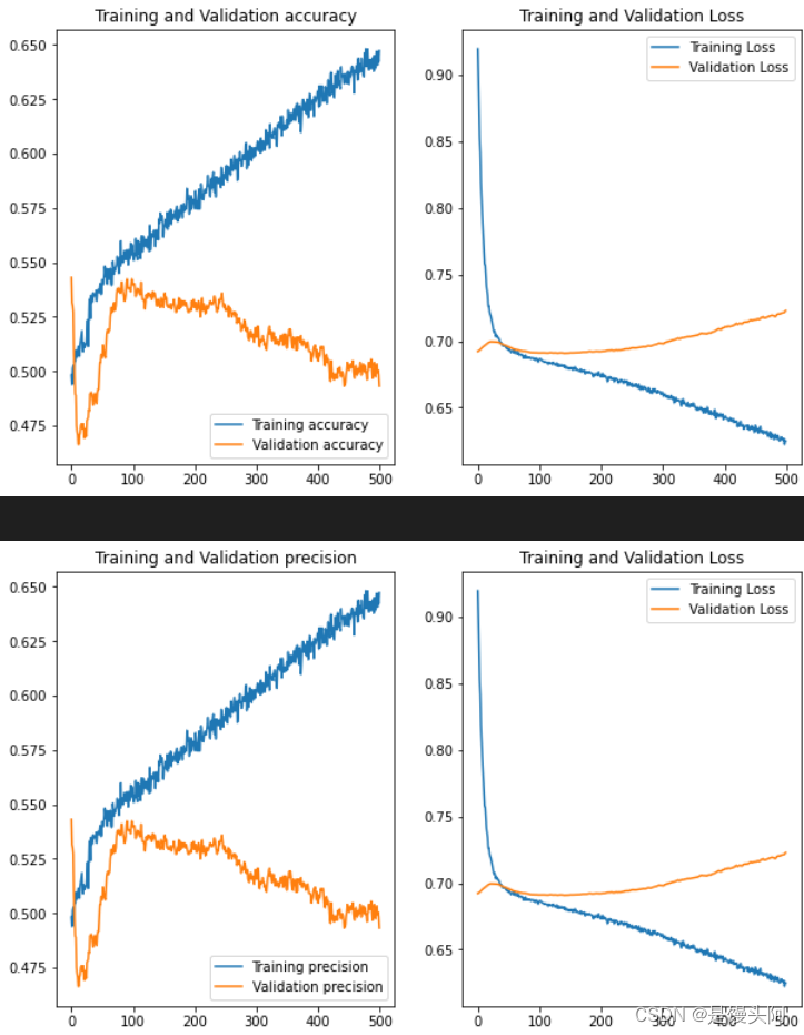
10.1 第一次验证
baseline_models = dummy_models(sub_signals = 12, metrics = METRICS)
history = [0]*32
epochs = 500
#range will be 32 in actual code
for j in range(1):
  print(f'Individual Net : {j+1}')
  x_train, x_val, y_train, y_val = train_test_split( X_train_12[j],y_train_12, test_size = 0.1, random_state = 42, shuffle = True, stratify = y_train_12)

  #Input Dependent dummy model
  history[j] = baseline_models[j].fit(x_train, y_train, batch_size = 2048, epochs = epochs, \
                                      validation_data = (x_val, y_val), shuffle = True, verbose = 0)

  show_metrics(x_train, x_val, y_train, y_val, baseline_models[j])
  show_test_metrics(x_test_12[j], y_test_12, baseline_models[j])

  plot_evaluation_curves(history[j], epochs, ('accuracy', 'val_accuracy'))
  plot_evaluation_curves(history[j], epochs, ('precision', 'val_precision'))
  plot_evaluation_curves(history[j], epochs, ('recall', 'val_recall'))
  plot_evaluation_curves(history[j], epochs, ('auc', 'val_auc'))
  print("\n-----------------------------------------------------------------------------------------")
  baseline_models[j].save("/content/drive/MyDrive/major project/1D-CNN Models/Vanilla Models/bin_12_baseline")
  gc.collect()
gc.collect()
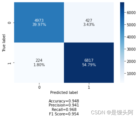

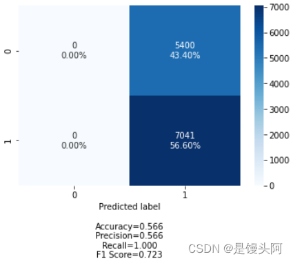
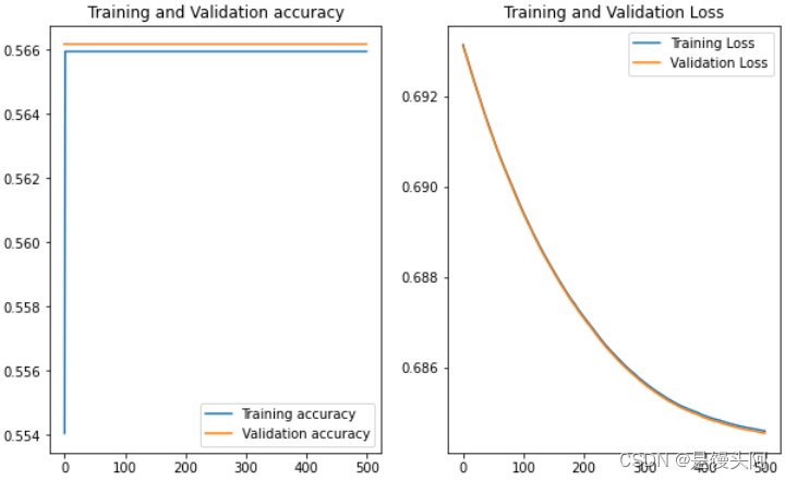
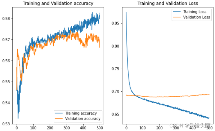
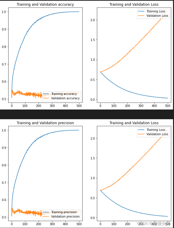
ACC+Loss
PR+Loss

RE+Loss

AUC+Loss


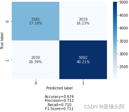
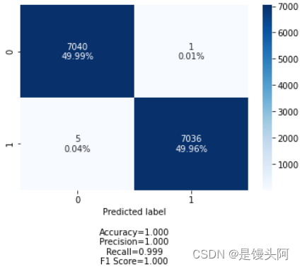
还是炸了,但模型训练好了,未过拟合,train和test的acc炸了,裂开,在这想配个表情包,方便起见,下面我只贴出train和test的ACC+Loss对比,其他图和代码不贴了。还是不死心,再试试其他被试数据。
10.2 第二次尝试

害,您可别说,这个更离谱!再来!
10.3 第三次尝试
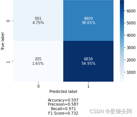

嗯......这次的train和test还算正常些,在这我总结了一下自己创建模型的坑,我们就像上帝之手,创建一个前所未有的模型就像创造生命,一开始上帝也不知道人应该是啥,都是慢慢摸索过来的,创建的人和搭建的模型缺鼻子少眼是不行的,下面是第四次探索。
10.4 第四次探索


test acc在上升!再来!
10.5 第五次拼搏

当场无语了,是第一种情况了,再来吧。
10.6 第六次终极无敌分析

结语:
经过六次模型探索,前面两个问题我心里有了答案,其中一个是,若是自己建立模型,遇到的坑是很多的,并最终模型分类精度在60%左右,我在STEW数据上建立的CNN也是如此。最后若有大神有自己建立模型的心得体会,欢迎留言交流学习。
