图像尺寸测量

写在前沿：
这部分，我自己还没完全弄懂，有些地方还未理解。写下来是因为，放在这上面，我会抽时间回来看看，然后进行补充，放在这里，主要是给自己提个醒，并且之后弄懂了，也会将其一些函数用法，已经其原理进行一一阐述。

1.导入相关库

from scipy.spatial import distance as dist
#导入imutils库，以及该库的perspective模块和contours模块，用于图像处理。
import imutils
from imutils import perspective
from imutils import contours
#导入numpy用于创建数组，cv2用于图像处理。
import numpy as np
import cv2
import matplotlib.pyplot as plt

2.读取参照物和待测物

参照物img_reference

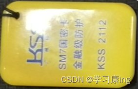
image

# 读取参照物, 比例不能缩放
img_reference = cv2.imread('yaoshi2.jpg')
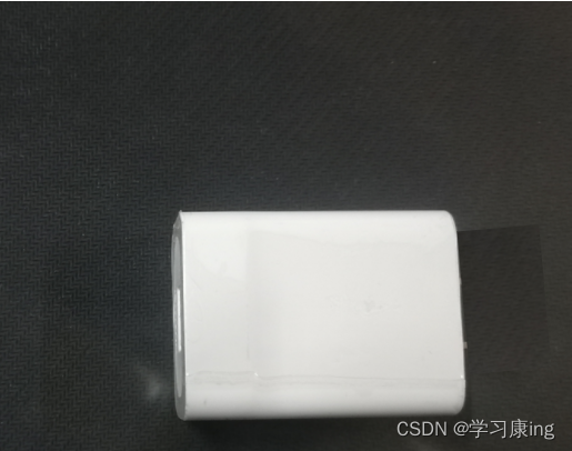
# 读取需要呗测量的物体
image = cv2.imread('yaoshi3.jpg')
if not image.data:  # 检查是否读入图片
    print("read image wrong!")
if not img_reference.data:
    print("read img_reference wrong")

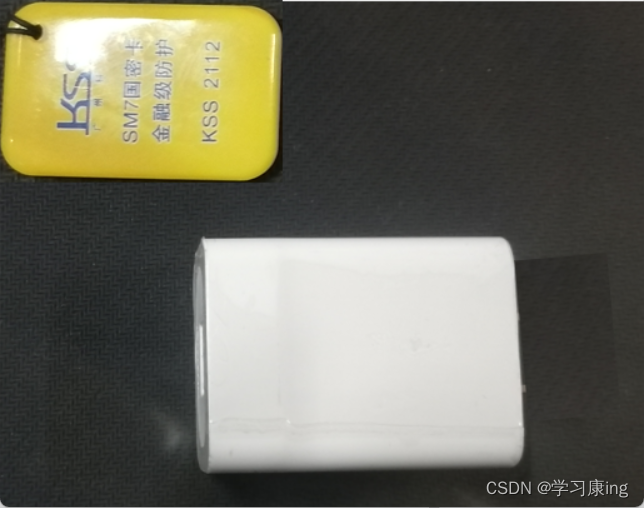
# 图像混合
# 创建空三维数组用来储存参照物
rows,cols,channels = img_reference.shape
# 将参照物放进刚才创建的二维数组
rio = image[0:rows,0:cols]
# 将图片的左上角换成参照物
res = cv2.addWeighted(img_reference, 1, rio, 0, 0)

dst1 = image.copy()#对原图像进行拷贝
dst1[0:rows,0:cols] = res
#展示
cv2.imshow('dst1',dst1)
cv2.waitKey()
cv2.destroyAllWindows()

这里的图像混合我在前面的的文件和总结都用过
cv2.addWeighted(img_reference, 1, rio, 0, 0)
1代表img_reference的权重比，1代表全是img_reference
第一个0代表rio的权重比，0表示完全被覆盖
第二个0代表其rio的亮度

3图像处理

高斯滤波：

• cv2.GaussianBlur(src, ksize, sigmaX)，返回与原图相同尺寸变得更清晰的图
• src：输入图像
• ksize：高斯核大小
• sigmaX：X方向上的高斯核标准偏差

边缘检测：

• cv2.Canny(image, threshold1, threshold2)，返回一副二值图，其中包含检测出的边缘
• image：需要处理的原图像，该图像必须为单通道的灰度图
• threshold1：阈值1
• threshold2：阈值2
  较大的阈值2用于检测图像中明显的边缘，但一般情况下检测的效果不会那么完美，边缘检测出来是断断续续的。所以这时候用较小的第一个阈值用于将这些间断的边缘连接起来

膨胀去噪

dilate = cv2.dilate(imgray, None, iterations=1)

腐蚀去噪

erosion = cv2.erode(dilate, None, iterations=1)

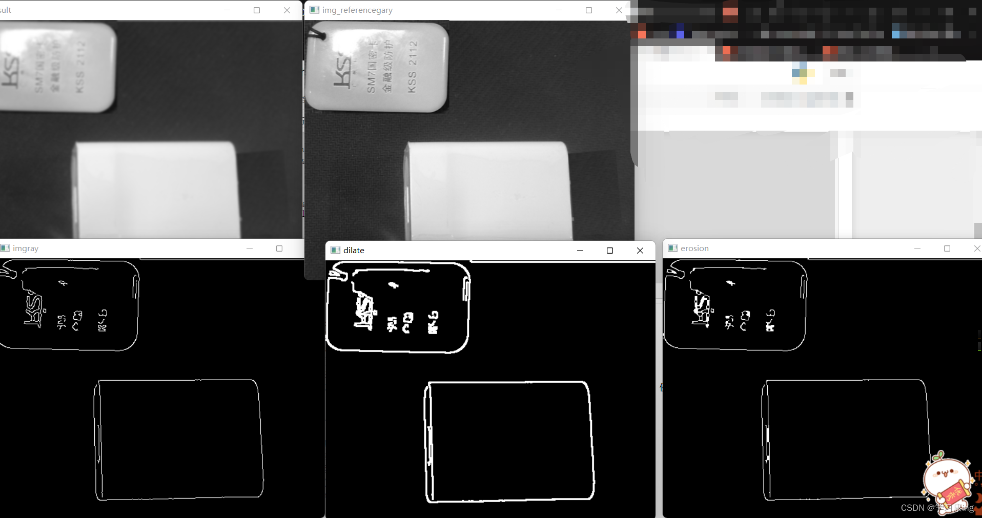
正文

# 加载图像，将其转换为灰度，然后稍微模糊
img_referencegary = cv2.cvtColor(dst1, cv2.COLOR_BGR2GRAY)
cv2.imshow('img_referencegary',img_referencegary)
cv2.waitKey()

# 高斯滤波，图像变得更清晰
result = cv2.GaussianBlur(img_referencegary,(7,7), sigmaX=0, sigmaY=0)
cv2.imshow('result',result)
cv2.waitKey()

# 执行边缘检测，然后执行膨胀+腐蚀以闭合对象边缘之间的间隙
# 边缘检测
imgray = cv2.Canny(result, 50,100)
cv2.imshow('imgray',imgray)
cv2.waitKey()

# 膨胀去噪
dilate = cv2.dilate(imgray, None, iterations=1)
cv2.imshow('dilate',dilate)
cv2.waitKey()

# 腐蚀去噪
erosion = cv2.erode(dilate, None, iterations=1)
cv2.imshow('erosion',erosion)
cv2.waitKey()
cv2.destroyAllWindows()

4 轮廓检测并初始化变量

轮廓检测：

• cv2.findContours(image, mode, method)参数说明如下。
• image：接受的参数为二值图，即黑白的（不是灰度图）
• mode：cv2.RETR_EXTERNAL表示只检测外轮廓
• method：cv2.CHAIN_APPROX_SIMPLE压缩水平方向，垂直方向，对角线方向的元素，只保留该方向的终点坐标，例如一个矩形轮廓只需4个点来保存轮廓信息

轮廓获取可调用imutils.grab_contours(cnts)函数实现，其中cnts为轮廓检测的返回值。

实现轮廓检测并设定尺寸测量的初始化变量。

# 图形的轮廓检测
edged = erosion.copy()
cnts = cv2.findContours(edged,cv2.RETR_EXTERNAL,cv2.CHAIN_APPROX_SIMPLE)

cnts = imutils.grab_contours(cnts)  # 获取 cnts中的 countors(轮廓)

# print(cnts)
# 从左到右对轮廓进行排序，并初始化“pixels_per_metric”校准变量
# 返回已排序轮廓和边界框的列表
(cnts,boundingBoxes) = contours.sort_contours(cnts)


# 初始化比例系数
pixelsPerMetric = None

# 本代码使用的参照物自己拍照的门禁钥匙
width = 3
# 参照物的宽度(注意：是width，不是 height)，单位：cm

5 绘制轮廓并检测真实长度***

计算闭合轮廓的面积可使用cv2.contourArea(cnts)函数，其中cnts为检测到的轮廓。

获取包含点集的最小矩形框和矩形框的四个顶点，主要使用cv2.minAreaRect©和cv2.boxPoints(box)两个函数，其中cv2.minAreaRect(cnts)的参数为检测到的轮廓，cv2.boxPoints(box)的参数为cv2.minAreaRect()的返回值，而这两个函数一般结合使用。

通过for循环遍历轮廓点集，并在循环里绘制所检测的轮廓和实现真实长度的测量。

def midpoint(A, B):
    return ((A[0] + B[0]) * 0.5, (A[1] + B[1]) * 0.5)
# loop over the contours individually--分别在轮廓上循环
for c in cnts:
    # if the contour is not sufficiently large, ignore it--如果轮廓不够大，请忽略它
    if cv2.contourArea(c) < 100:
        continue

    # compute the rotated bounding box of the contour--计算轮廓的旋转边界框
    
    orig = image.copy()
    
    box = cv2.minAreaRect(c)
    # 求能包含点集的最小矩形框
    box = cv2.boxPoints(box)
    # 求矩形框的四个顶点
    box = np.array(box, dtype="int")


    # 对轮廓中，根据点的x坐标对点进行排序，使其以左上、右上、右下和左下的顺序出现，然后绘制旋转边界的轮廓
    # box return the coordinates in top-left, top-right,bottom-right, and bottom-left order
    box = perspective.order_points(box)

    cv2.drawContours(orig, [box.astype("int")], -1, (0, 255, 0), 2)
#cv2.drawContours(image, contours, contourIdx, color, thickness=None, lineType=None, hierarchy=None, maxLevel=None, offset=None)
#第一个参数是指明在哪幅图像上绘制轮廓；image为三通道才能显示轮廓
#第二个参数是轮廓本身，在Python中是一个list;
#thickness参数指定绘制轮廓list中的哪条轮廓，如果是-1，则绘制其中的所有轮廓。
#其中thickness表明轮廓线的宽度如果是-1（cv2.FILLED），则为填充模式。

    # 在原始点上循环并绘制它们
    for (x, y) in box:
        cv2.circle(orig, (int(x), int(y)), 5, (0, 0, 255), -1)#-1四个原点的填充

    # unpack the ordered bounding box,
    # then compute the midpoint between the top-left and top-right coordinates,
    # followed by the midpoint between bottom-left and bottom-right coordinates
    # 打开有序边界框，然后计算左上角和右上角坐标之间的中点，然后计算左下角和右下角坐标之间的中点
    (tl, tr, br, bl) = box
    (tltrX, tltrY) = midpoint(tl, tr)
    (blbrX, blbrY) = midpoint(bl, br)
    
    # compute the midpoint between the top-left and top-right points,
    # followed by the midpoint between the top-righ and bottom-right
    # 计算左上角点和右上角点之间的中点，然后计算右上角点和右下角点之间的中点
    (tlblX, tlblY) = midpoint(tl, bl)
    (trbrX, trbrY) = midpoint(tr, br)

    # draw the midpoints on the image--画出线段的中点
    cv2.circle(orig, (int(tltrX), int(tltrY)), 5, (255, 0, 0), -1)
    cv2.circle(orig, (int(blbrX), int(blbrY)), 5, (255, 0, 0), -1)
    cv2.circle(orig, (int(tlblX), int(tlblY)), 5, (255, 0, 0), -1)
    cv2.circle(orig, (int(trbrX), int(trbrY)), 5, (255, 0, 0), -1)

    # draw lines between the midpoints--在中点之间画线
    cv2.line(orig, (int(tltrX), int(tltrY)), (int(blbrX), int(blbrY)), (255, 0, 255), 2)
    cv2.line(orig, (int(tlblX), int(tlblY)), (int(trbrX), int(trbrY)), (255, 0, 255), 2)

    # compute the Euclidean distance between the midpoints
    # 计算中点之间的欧几里德距离
    dA = dist.euclidean((tltrX, tltrY), (blbrX, blbrY))
    dB = dist.euclidean((tlblX, tlblY), (trbrX, trbrY))
    
    # if the pixels per metric has not been initialized, then
    # compute it as the ratio of pixels to supplied metric
    # (in this case, inches)
    # 如果每个度量的像素尚未初始化，则将其计算为像素与提供的度量的比率(cm)
    if pixelsPerMetric is None:
        pixelsPerMetric = dB / width

    # compute the size of the object--计算对象的大小
    dimA = dA / pixelsPerMetric
    dimB = dB / pixelsPerMetric

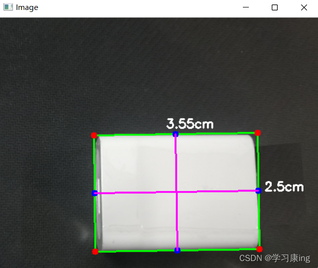
    # draw the object sizes on the image--在图像上绘制对象大小
    # in: 英寸, 1 in = 25.4 mm, 1 mm = 0.03937 in
    cv2.putText(orig, "{
    
    :.2f}cm".format(dimB),  # 长
                (int(tltrX - 15), int(tltrY - 10)), cv2.FONT_HERSHEY_SIMPLEX, 0.65, (255, 255, 255), 2)
    cv2.putText(orig, "{
    
    :.1f}cm".format(dimA),
                (int(trbrX + 10), int(trbrY)), cv2.FONT_HERSHEY_SIMPLEX,0.65, (255, 255, 255), 2)
    cv2.imshow("Image", orig)
    cv2.waitKey(0)
    cv2.destroyAllWindows()

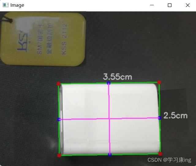
6 展示检测的图片

# 将左上角被替换为参照物的位置恢复
rows,cols,channels = orig.shape

rio = dst1[0:rows,0:cols]

res = cv2.addWeighted(orig, 0.6, rio, 0.4, 0)

dst2 = image.copy()#对原图像进行拷贝
dst2[0:rows,0:cols] = res


cv2.imshow("Image", dst2)
cv2.waitKey(0)
cv2.destroyAllWindows()

7 定义闭合轮廓的面积计算函数

自定义闭合轮廓面积的计算函数contourArea()，设定轮廓参数为cnt。

def contourArea(cnt):  # 传入一个轮廓
    # 最小外接矩形
    rect = cv2.minAreaRect(cnt)
    # 求矩形的四个顶点
    
    box = cv2.boxPoints(rect)
    box = np.int0(box)

    return cv2.contourArea(box)  # 计算闭合轮廓的面积

8 定义面积测量函数

自定义measure_object()函数用于计算测量面积。

def measure_object(image):
    gray = cv2.cvtColor(image, cv2.COLOR_BGR2GRAY)  # 灰度化
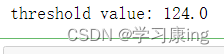
    ret, binary = cv2.threshold(gray, 0, 255, cv2.THRESH_BINARY | cv2.THRESH_OTSU)  # 二值化(cv.THRESH_OTSU: 自动求出最优阈值)
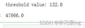
    # 打印阈值
    print("threshold value: %s"%(ret)) #分割的阈值
    # 展示二值化图片
    cv2.imshow('binary',binary)
    cv2.waitKey(0)
    cv2.destroyAllWindows()
    contours, hierarchy = cv2.findContours(binary, cv2.RETR_EXTERNAL, cv2.CHAIN_APPROX_SIMPLE)  # 检测轮廓
    #print(contours)
    for contour in contours:
    
        if cv2.contourArea(contour)<100:# 如果轮廓不够大，则舍去，我们只检测拥有一定轮廓的物体
            continue
        area = contourArea(contour)
    return  area

9 计算参照物和被检测物体的面积

# 参照物像素计算
img_reference = cv2.imread('yaoshi2.jpg')

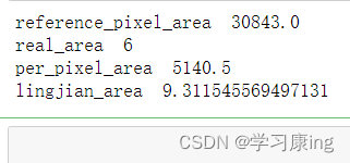
reference_pixel_area =  measure_object(img_reference) # 参照物像素：30843.0
#print('参照物像素：',reference_pixel_area)

# 计算其真实面积, # 6
real_area = width*2
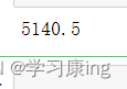
# 求每个像素占多少面积: 像素 / 真实面积
per_pixel_area =  reference_pixel_area/real_area
print(per_pixel_area)
# 5140.5

# 被测零件像素计算
img = cv2.imread('yaoshi3.jpg')
img_area =  measure_object(img) 
lingjian_area = img_area/per_pixel_area
img_area
# 真实物像素：47866.0

# 9.311545569497131
print('reference_pixel_area ',reference_pixel_area)
print('real_area ',real_area)
print('per_pixel_area ',per_pixel_area)
print('lingjian_area ',lingjian_area)

总的来说不简单，第四部分我自己还有还有部分没弄清楚，后续会在这篇文件上去更改
其余部分基本上不难，一些点我都进行了分析和注释，最重要的是理解每个函数到底是干什么用，后续会对这些函数进行一个总结，基本上会1-2节总结一次，也许有些总结都是重复的，但是看得越多也就能记得越多啦。