一、YOLOV5训练数据基本格式以及格式的相互转换(labimg标注数据格式)
1.1 VOC数据格式
基本图片数据集,每张图片对应的.xml标注文件,类别classes.txt文件。
其中.xml的具体结构如下所示:
<annotation>
	<folder>tupian3</folder>
	<filename>1.jpg</filename>
	<path>C:\Users\hp\Desktop\tupian3\1.jpg</path>     // 该标注文件对应的原图路径
	<source>
		<database>Unknown</database>
	</source>
	<size>
		<width>2448</width>                             // 图像的长宽和通道数
		<height>2048</height>
		<depth>3</depth>
	</size>
	<segmented>0</segmented>
	<object>
		<name>slider</name>                           // 类别标签1
		<pose>Unspecified</pose>
		<truncated>0</truncated>
		<difficult>0</difficult>
		<bndbox>                                    // 类别标签目标1对应的左上角和右下角坐标
			<xmin>941</xmin>
			<ymin>837</ymin>
			<xmax>2007</xmax>
			<ymax>1462</ymax>
		</bndbox>
	</object>
	<object>
		<name>table</name>                      // 类别标签2
		<pose>Unspecified</pose>
		<truncated>0</truncated>
		<difficult>0</difficult>
		<bndbox>
			<xmin>302</xmin>                     // 类别标签2对应的目标1对应的左上角和右下角坐标
			<ymin>555</ymin>
			<xmax>904</xmax>
			<ymax>787</ymax>
		</bndbox>
	</object>
	<object>
		<name>table</name>
		<pose>Unspecified</pose>
		<truncated>0</truncated>
		<difficult>0</difficult>
		<bndbox>
			<xmin>323</xmin>                     // 类别标签2对应的目标2对应的左上角和右下角坐标
			<ymin>1505</ymin>
			<xmax>875</xmax>
			<ymax>1721</ymax>
		</bndbox>
	</object>
</annotation>
1.2 YOLO数据格式
包含标注原图像,标注.txt文件且每个文件名与原图像名称一致,标签类别.txt文件。
.txt文件的具体类容如下:[x_center, y_center, width, height]
0 0.604371 0.561279 0.438317 0.305176
1 0.248775 0.325928 0.239379 0.109863
1 0.245507 0.786133 0.227124 0.111328
// 0/1 表示类别  , 后面依次是归一化后的中心点以及宽高。
1.3 CreatML数据格式
包含原始图像数据集,标注文件.json且文件序号与原图像序号一致,类别标签文件.txt
[{"image": "1.jpg",
 "annotations": [
 	{"label": "s",
 		"coordinates": {"x": 1479.818181818182, "y": 1140.8636363636363, "width": 1063.0, "height": 620.9999999999999}},
	{"label": "c",
		"coordinates": {"x": 337.8181818181819, "y": 1131.8636363636363, "width": 210.99999999999997, "height": 203.0}},
	{"label": "c",
		"coordinates": {"x": 2302.318181818182, "y": 1170.8636363636363, "width": 118.0, "height": 111.0}},
    {"label": "t",
    	"coordinates": {"x": 604.818181818182, "y": 670.3636363636364, "width": 591.0, "height": 230.0}},
   	{"label": "t",
   		"coordinates": {"x": 601.318181818182, "y": 1614.8636363636363, "width": 566.0, "height": 219.0}}
 	]
 }]

// 上面的标注格式依次为:原图像路径
// annotations标注数据:标签类别s -  s类目标1的中心坐标和宽高 - s类目标2的中心坐标和宽高
1.4 CoCo的基本数据格式
**[x_min, y_min, width, height]**
1.5 实现将CreatMl和voc格式转换为yolo格式的python代码
- 实现将VOC数据格式转换为YOLO格式
def read_xml(xml_path):
    tree = xmlET.parse(xml_path)
    size = tree.find('size')   # 获取图片尺寸字段
    width = int(size.find('width').text)
    height = int(size.find('height').text)
    image_path = str(tree.find('filename').text)

    # 目标字段
    obj_s = tree.findall('object')
    bnd_box = []   # 存储一张图片中所有类别的目标框[xmin,ymin,xmax,ymax,label]
    for obj in obj_s:
        label = obj.find("name").text
        bnd = obj.find("bndbox")
        xmin = int(bnd.find("xmin").text)
        ymin = int(bnd.find("ymin").text)
        xmax = int(bnd.find("xmax").text)
        ymax = int(bnd.find("ymax").text)
        bbox = [xmin, ymin, xmax, ymax, label]
        bnd_box.append(bbox)
    return [[width, height, image_path], bnd_box]
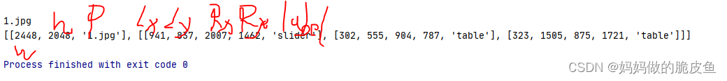
存储顺序:图像宽高路径,目标框左上和右下坐标,类别标签
- 实现将COCO数据格式转换为YOLO格式
// 读取单个.json文件
def read_xml(xml_path):
    tree = xmlET.parse(xml_path)
    size = tree.find('size')   # 获取图片尺寸字段
    width = int(size.find('width').text)
    height = int(size.find('height').text)
    image_path = str(tree.find('filename').text)

    # 目标字段
    obj_s = tree.findall('object')
    bnd_box = []   # 存储一张图片中所有类别的目标框[xmin,ymin,xmax,ymax,label]
    for obj in obj_s:
        label = obj.find("name").text
        bnd = obj.find("bndbox")
        xmin = int(bnd.find("xmin").text)
        ymin = int(bnd.find("ymin").text)
        xmax = int(bnd.find("xmax").text)
        ymax = int(bnd.find("ymax").text)
        bbox = [xmin, ymin, xmax, ymax, label]
        bnd_box.append(bbox)
    return [[width, height, image_path], bnd_box]
返回结果如下图所示:
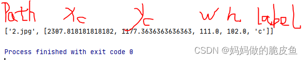
存储顺序为:图像路径,目标框中心坐标以及宽高和类别标签。
- 完整代码如下所示(部分代码较上面做了些许调整,注意下面转化后的yolo数据并没有将类别标签转换为对应的数字标签,存储的.txt的文件名就是图像的名称):
import numpy as np
import os, random, json
import xml.etree.ElementTree as xmlET
import json
import cv2


def mkdir(path):
    if not os.path.exists(path):
        os.makedirs(path)
        return True
    else:
        print(f"The path ({

      path}) already exists.")
        return False


# 返回一张图片中所有类别标签标注的列表,数据格式为:[[xmin,ymin,xmax,ymax,label],[xmin,ymin,xmax,ymax,label],......]
def read_xml(xml_path):
    tree = xmlET.parse(xml_path)
    size = tree.find('size')   # 获取图片尺寸字段
    width = int(size.find('width').text)
    height = int(size.find('height').text)
    image_path = str(tree.find('filename').text)

    # 目标字段
    obj_s = tree.findall('object')
    bnd_box = []   # 存储一张图片中所有类别的目标框[xmin,ymin,xmax,ymax,label]
    for obj in obj_s:
        label = obj.find("name").text
        bnd = obj.find("bndbox")
        xmin = int(bnd.find("xmin").text)
        ymin = int(bnd.find("ymin").text)
        xmax = int(bnd.find("xmax").text)
        ymax = int(bnd.find("ymax").text)
        # 还是要进行归一化处理的
        width_nor = (xmax - xmin) * (1 / float(width))
        height_nor = (ymax - ymin) * (1 / float(height))
        center_x = (xmin + xmax)/ 2. * (1 / float(width))
        center_y = (ymin + ymax)/ 2. * (1 / float(height))
        bbox = [label, center_x, center_y, width_nor, height_nor]
        bnd_box.append(bbox)
    return [[width, height, image_path], bnd_box]


# 返回一张图片中所有类别标签标注的列表,数据格式为:[[xmin,ymin,xmax,ymax,label],[xmin,ymin,xmax,ymax,label],......]
def read_json(json_path, img_width, img_height):   # 读取coco数据标注文件.json
    with open(json_path) as f:
        data = json.load(f)     # 包含‘image’和 'annotations'两个键
    data_annotation = data[0]['annotations']
    image_path = data[0]['image']

    num_obj = len(data_annotation)
    bnd_box = []   # 用于存储所有的目标框数据
    for obj in data_annotation:
        label = obj['label']
        value_coord = obj['coordinates']
        center_x = value_coord['x'] / float(img_width)
        center_y = value_coord['y'] / float(img_height)
        width = value_coord['width'] / float(img_width)
        height = value_coord['height'] / float(img_height)

        bbox = [label, center_x, center_y,width,height]
        bnd_box.append(bbox)
    return [image_path, bnd_box]


# 读取存储.xml的目录下的所有.xml文件,并将结果存储到指定的目录下xml_dir= "C:/Users/hp/Desktop/1/"; yolo_save_dir = "C:/Users/hp/Desktop/2/"
def xmlToYolo(xml_dir, yolo_save_dir):
    files = os.listdir(xml_dir)
    for subFile in files:  # 遍历.xml文件
        file_path = os.path.join(xml_dir, subFile)  # 拼接文件绝对路径,最好不要使用中文目录,若为中文。unicode(path,'utf-8')
        if os.path.exists(file_path):
            per_list = read_xml(file_path)   # 返回每张图片标注的目标框
            # 拆分图像名称,并将数字部分作为.txt的文件名
            img_name = str(per_list[0][2])
            new_txt_name = os.path.join(yolo_save_dir, str(img_name.split('.')[0])+'.txt')
            f = open(new_txt_name,"w")
            len_box = len(per_list[1])
            for i in range(len_box):
                for j in range(len(per_list[1][i])):
                    per_box = per_list[1][i]
                    per_value = per_box[j]
                    if j != 0:
                        per_value = format(per_value, '.3f')
                    f.write(str(per_value))
                    if j < len(per_list[1][i]) -1:
                        f.write(" ")
                if i < len_box - 1:
                    f.write("\n")
            f.close()


def jsonToYolo(json_dir, yolo_save_dir):
    files = os.listdir(json_dir)
    for subFile in files:  # 遍历.xml文件
        file_path = os.path.join(json_dir, subFile)  # 拼接文件绝对路径,最好不要使用中文目录,若为中文。unicode(path,'utf-8')
        if os.path.exists(file_path):
            per_list = read_json(file_path, 2448, 2048)  # 返回每张图片标注的目标框,这里需要传入自己的图片宽高
            img_name_id = str(per_list[0]).split('.')[0]
            new_txt_name = os.path.join(yolo_save_dir, str(img_name_id) + '.txt')
            f = open(new_txt_name,"w")
            len_box = len(per_list[1])
            for i in range(len_box):
                for j in range(len(per_list[1][i])):
                    per_box = per_list[1][i]
                    per_value = per_box[j]
                    if j != 0:
                        per_value = format(per_value, '.3f')   # 只保留三位小数点
                    f.write(str(per_value))
                    if j < len(per_list[1][i]) -1:
                        f.write(" ")
                if i < len_box - 1:
                    f.write("\n")
            f.close()


# 是将所有的.json文件转换为yolo,并存储在指定的目录下
# def cocoToYolo(json_dir, yolo_dir):
# Press the green button in the gutter to run the script.
if __name__ == '__main__':
    # 1. 实现将voc的.xml转换为yolo的.txt标注数据
    xmlToYolo("C:/Users/hp/Desktop/1", "C:/Users/hp/Desktop/2")

    # 2. 实现将coco的.json文件转换为yolo的.txt文件
    jsonToYolo("C:/Users/hp/Desktop/3", "C:/Users/hp/Desktop/4")
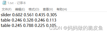
结果展示,在数据处理过程中一定要注意.txt中的空格以及换行符,容易在训练过程中造成数据的读写错误:
二、环境搭建以及模型选择
环境搭建过程,在此省略。
2.1 YOLOV5甚至其他YOLO系列更高版本模型的选择
本文选择:yolov5l.yaml模型结构
基本结构:
# Parameters
nc: 80  # number of classes
depth_multiple: 1.0  # model depth multiple
width_multiple: 1.0  # layer channel multiple
anchors:
  - [10,13, 16,30, 33,23]  # P3/8
  - [30,61, 62,45, 59,119]  # P4/16
  - [116,90, 156,198, 373,326]  # P5/32

# YOLOv5 v6.0 backbone
backbone:
  # [from, number, module, args]
  [[-1, 1, Conv, [64, 6, 2, 2]],  # 0-P1/2
   [-1, 1, Conv, [128, 3, 2]],  # 1-P2/4
   [-1, 3, C3, [128]],
   [-1, 1, Conv, [256, 3, 2]],  # 3-P3/8
   [-1, 6, C3, [256]],
   [-1, 1, Conv, [512, 3, 2]],  # 5-P4/16
   [-1, 9, C3, [512]],
   [-1, 1, Conv, [1024, 3, 2]],  # 7-P5/32
   [-1, 3, C3, [1024]],
   [-1, 1, SPPF, [1024, 5]],  # 9
  ]

# YOLOv5 v6.0 head
head:
  [[-1, 1, Conv, [512, 1, 1]],
   [-1, 1, nn.Upsample, [None, 2, 'nearest']],
   [[-1, 6], 1, Concat, [1]],  # cat backbone P4
   [-1, 3, C3, [512, False]],  # 13

   [-1, 1, Conv, [256, 1, 1]],
   [-1, 1, nn.Upsample, [None, 2, 'nearest']],
   [[-1, 4], 1, Concat, [1]],  # cat backbone P3
   [-1, 3, C3, [256, False]],  # 17 (P3/8-small)

   [-1, 1, Conv, [256, 3, 2]],
   [[-1, 14], 1, Concat, [1]],  # cat head P4
   [-1, 3, C3, [512, False]],  # 20 (P4/16-medium)

   [-1, 1, Conv, [512, 3, 2]],
   [[-1, 10], 1, Concat, [1]],  # cat head P5
   [-1, 3, C3, [1024, False]],  # 23 (P5/32-large)

   [[17, 20, 23], 1, Detect, [nc, anchors]],  # Detect(P3, P4, P5)
  ]
2.2 搭建深度学习模型
2.2.1 数据增强策略与代码实现(一般工业中检测目标相对单一且环境稳定,所以不需要过于复杂的增强策略)
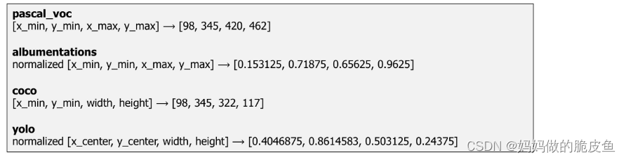
2.2.1.1 图像增强开源库Albumentations的基础用法
Albumentations是一个强大的开源图像增强库,那么对于目标检测任务,如何获取变化后图像的对应标注的groundbox呢?下面就写一个数据增强的方法,主要用于生成哪些会改变标签坐标的增强方法:
Albumentations支持四种目标检测标注格式pascal_voc、albumentations、coco、yolo;具体格式如下图所示:
对目标检测任务的图像增强基本包含4个步骤:
- 导入需要的库
- 定义一个增强管道
- 从硬盘中读取图像和对应的标注框
- 传递图像和标注框给数据管道并返回增强后的图像和新的标注框。
import albumentations as A
import cv2
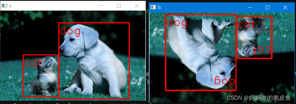
def AgumentaitionAndLabel():
# step1: 声明增强数据管道
transform = A.Compose([
# A.RandomCrop(width=450, height=450),
A.HorizontalFlip(p=0.8),
A.VerticalFlip(p=0.8),
A.RandomBrightnessContrast(p=0),
], bbox_params=A.BboxParams(format='pascal_voc')) # 其他类型的标注数据格式,需要将下面的bboxes按照上面图标格式进行转换即可
# step2:读取图像数据和标签数据
image = cv2.imread("C:/Users/Administrator/Desktop/12.jpg")
image = cv2.cvtColor(image, cv2.COLOR_BGR2RGB)
size = image.shape
bboxes = [
[154, 32, 340, 233, 'dog'],
[60, 117, 153, 228, 'cat']
]
for per in bboxes:
cv2.putText(image, per[4], (int(per[0]), int(per[1])+30), cv2.FONT_HERSHEY_DUPLEX, 1, (0, 0, 255), 1)
cv2.rectangle(image, (int(per[0]), int(per[1])), (int(per[2]), int(per[3])), (0, 0, 255), 2)
cv2.imshow("a", image)
# step3: 传入图像和标签实现数据增强,同时返回增强图像和增强图像的标注box
transformed = transform(image=image, bboxes=bboxes)
transformed_image = transformed['image']
transformed_bboxes = transformed['bboxes']
for per in transformed_bboxes:
cv2.putText(transformed_image, per[4], (int(per[0]), int(per[1])+30), cv2.FONT_HERSHEY_DUPLEX, 1, (0, 0, 255), 1)
cv2.rectangle(transformed_image, (int(per[0]), int(per[1])), (int(per[2]), int(per[3])), (0, 0, 255), 2)
cv2.imshow("b", transformed_image)
cv2.waitKey(0)
if __name__ == '__main__':
AgumentaitionAndLabel()
函数的参数解释:
bbox_params=A.BboxParams(format='coco', min_area=1024, min_visibility=0.1, label_fields=['class_labels'])
# min_area ----表示增强后的标注框的面积的最小值,如果小于该值就舍弃该增强包围框;
# min_visibility---表示增强后的标注框的面积与原始标注框面积的比值,如果增强后包围框的比值比设定阈值小,那么就舍弃该增强后的标注框。
# label_fields---为边界框传递标签,这里支持两种传递标签的方式
# 传递标签方式1:[23, 74, 295, 388, 'dog']/[23, 74, 295, 388, 18-类别标签]将标签与坐标一起传递(一个框可以包含多个类别:[23, 74, 295, 388, 'dog', 'animal'])
# 传递标签方式2:类别与坐标分开传递--[23, 74, 295, 388][377, 294, 252, 161][333, 421, 49, 49]['cat', 'dog', 'sports ball'][18, 17, 37]
以上内容的参考地址:详细描述了Albumentations如何应用于目标检测任务中
具体官方案例
当然在实际工程中,往往更偏向与进行实时的数据增强处理,而不是先对源图像进行增强处理,将增强数据保存到硬盘,再去读取进行深度学习模型的训练。为了将Albumentations和具体的深度学习框架的数据管道紧密结合在一起,通常使用如下的操作:
这一过程的关键在于如何将增强数据结果转换为对应深度学框架下的数据类型:以pytorch为例,Albumentations提供了ToTensorV2()函数,只需在声明数据管道对象时,将该函数作为参数传递即可,具体格式如下所示:
# pytorch中构建数据处理类
class CatsVsDogsDataset(Dataset):
    def __init__(self, images_filepaths,all_boxs, transform=None):
        self.images_filepaths = images_filepaths
        self.transform = transform

    def __len__(self):
        return len(self.images_filepaths)

    def __getitem__(self, idx):
        image_filepath = self.images_filepaths[idx]
        image = cv2.imread(image_filepath)
        image = cv2.cvtColor(image, cv2.COLOR_BGR2RGB)
        bboxes = all_boxs[idx]
        transformed = self.transform(image=image, bboxes=bboxes)
	 	transformed_image = transformed['image']
		transformed_bboxes = transformed['bboxes']
        return transformed_image , transformed_bboxes

# Albumentations构建数据增强管道
train_transform = A.Compose(
    [
        A.SmallestMaxSize(max_size=160),
        A.ShiftScaleRotate(shift_limit=0.05, scale_limit=0.05, rotate_limit=15, p=0.5),
        A.RandomCrop(height=128, width=128),
        A.RGBShift(r_shift_limit=15, g_shift_limit=15, b_shift_limit=15, p=0.5),
        A.RandomBrightnessContrast(p=0.5),
        A.Normalize(mean=(0.485, 0.456, 0.406), std=(0.229, 0.224, 0.225)),
        ToTensorV2(),   # 这里是关键
    ]
)
train_dataset = CatsVsDogsDataset(images_filepaths=train_images_filepaths, all_boxs = boxs_lists, transform=train_transform)   # 将train_transform作为函数参数传递给pytorch中构建的数据管道中。
2.2.1.2 本工程中使用的图像处理方法
基本数据处理流程:
- 对标注原图像进行PAD操作,将非640的图像缩放至640,且保持原图像的长宽比:函数letterbox
- 根据对图像长宽的缩放比例,实现将原图像的标注框变换到pad后的图像上:函数 convert_yolo
- 使用Albumentations对pad图像进行更多的数据增强操作: 函数augment_image
- 注意:对于上面三个处理函数的所有功能只需要调用函数all_data_augmentation即可。
实现代码
# 该程序实现将yolo格式的数据进行图像增强和图像pad处理,并将对应的标签文件全部转换到对应的增强格式下
import cv2
import numpy as np
import os
import albumentations as A
import warnings
# step1: 先将加载的图像缩放大指定大小,并对小边进行pad操作
def letterbox(img, new_shape=(640, 640), color=(0, 0, 0), auto=True, scale_fill=False, scale_up=True, stride=32):
shape = img.shape[:2] # 获取图像当前的 [height, width]
if isinstance(new_shape, int): # 如果new_shape是整数,就将new_shape扩展为(640,640)
new_shape = (new_shape, new_shape) # new_shape = (640,640)
# 计算缩放比例,下面用于选出缩放比最小的那一条边,以保证按比例缩放不失真
r = min(new_shape[0] / shape[0], new_shape[1] / shape[1])
# 只进行下采样 因为上采样会让图片模糊
if not scale_up: # only scale down, do not scale up (for better test mAP)
r = min(r, 1.0)
# 计算需要填充的数量,ratio = 640/ current_w ; ratio = 640/ current_h
ratio = (r, r) # width, height ratios, 以其中最小的比例对长宽同时进行缩放操作。
# 先对宽进行缩放,再对高进行缩放, 从而得到新图象的宽高
new_unpad = int(round(shape[1] * r)), int(round(shape[0] * r))
# 计算非640的边需要填充多少行(dw, dh) padding
dw, dh = new_shape[1] - new_unpad[0], new_shape[0] - new_unpad[1]
# 进行最小填充,保证每条边都能被32整除,这是因为yolov5的下采样最大倍数就是32
if auto:
dw, dh = np.mod(dw, stride), np.mod(dh, stride)
# 其他的方式就是直接进行拉伸处理,会失真
elif scale_fill: # stretch
dw, dh = 0.0, 0.0
new_unpad = (new_shape[1], new_shape[0])
ratio = new_shape[1] / shape[1], new_shape[0] / shape[0] # width, height ratios
dw /= 2 # 宽方向填充数量
dh /= 2 # 高方向填充的数量
if shape[::-1] != new_unpad: # resize
img = cv2.resize(img, new_unpad, interpolation=cv2.INTER_LINEAR)
top, bottom = int(round(dh - 0.1)), int(round(dh + 0.1))
left, right = int(round(dw - 0.1)), int(round(dw + 0.1))
img = cv2.copyMakeBorder(img, top, bottom, left, right, cv2.BORDER_CONSTANT, value=color) # add border
return img, ratio, dw, dh # 返回的是pad后的图片,以及宽高比,dw,dh表示在宽和高上填充的数量。
# 如何将填充前图像的真实框扩展到当前填充后呢?以YOLO格式的图像为例[0, X_center, y_center, width, height]
def convert_yolo(box_data, image_source, image_pad, ratio, dw, dh):
"""
:param box_data: 标注数据,格式是yolo [0, X_center, y_center, width, height]都经过了归一化处理
:param image_source: 原始图像,用于提供原始图像的长宽,去恢复标注框的大小
:param image_pad: pad以及缩放后的图像,用于提供pad后图像的长宽
:param ratio: 提供pad图像的缩放比例(r,r)
:param dw: 宽方向填充的数量
:param dh: 长方向上提供的数量
:return: 返回矫正后的标注框
"""
h, w = image_source.shape[:2] # h,w
box_x, box_width = box_data[1] * w, box_data[3] * w
box_y, box_height = box_data[2] * h, box_data[4] * h
# 整体缩放Box的宽高
new_width, new_height = box_width * ratio[1], box_height * ratio[0]
# 移动box的中心点坐标
box_x, box_y = box_x * ratio[1], box_y * ratio[0]
box_x, box_y = box_x + dw, box_y + dh
# cv2.circle(image_pad,(int(box_x), int(box_y)),10, (0, 0, 255))
# pt1 = (int(box_x - new_width/2), int(box_y - new_height/2))
# pt2 = (int(box_x + new_width/2), int(box_y + new_height/2))
# cv2.rectangle(image_pad, pt1, pt2, (0, 0, 255))
class_id = box_data[0]
img_h, img_w = image_pad.shape[:2]
# 对计算的新值进行归一化处理
box_x, box_y, new_width, new_height = box_x/img_w, box_y/img_h, new_width/img_w, new_height/img_h
return [box_x, box_y, new_width, new_height, class_id]
# 进行图像增强处理, 可以自行添加相关增强方法的具体参数,使数据增强效果更丰富
def augment_image(image, label_yolo_label):
"""
---使用上下,左右随机翻转、以及添加噪声数据、改变对比度,混合通道---
:image: 输入图像
:label_yolo_label: 输入图像对应的标注数据, 是一个列表标签[x_center, y_center, width, height, labels]
:return: 返回增强后的图像,以及对应的标注数据
"""
transform = A.Compose([
A.HorizontalFlip(p=0.2), # 进行水平随机翻转
A.VerticalFlip(p=0.3), # 进行垂直翻转
A.RandomBrightnessContrast(p=0.4), # 随机亮度对比
A.Blur(p=0.2),
A.GaussNoise(p=0.3),
A.MedianBlur(p=0.3),
A.ChannelShuffle(p=0.3)
], bbox_params=A.BboxParams(format='yolo'))
transformed = transform(image=image, bboxes=label_yolo_label)
transformed_image = transformed['image']
transformed_boxes = transformed['bboxes']
return transformed_image, transformed_boxes
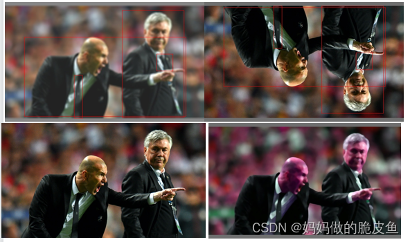
# 实现所有图像数据的增强处理,整个基础数据的处理只需调用该函数即可
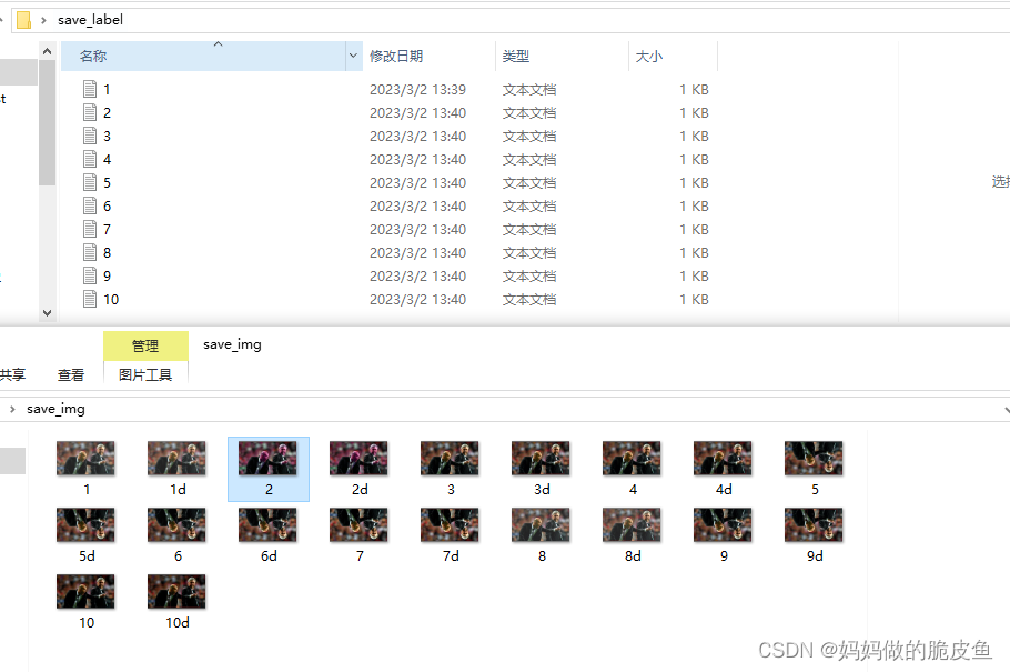
def all_data_augmentation(image_file, yolo_label_file, save_img_file, label_save_file, aug_epoch):
"""
:param image_file: 保存图像的文件夹的路径
:param yolo_label_file: 保存图像标注的文件路劲
:param save_img_file: 保存基础处理之后的图像文件夹
:param label_save_file: 保存基础处理后图像对应标注框的文件
:param aug_epoch: 表示进行多少个循环的图像增强处理
:return: 无返回值
"""
files_image = os.listdir(image_file) # 读取给定的图像存储文件夹
files_label = os.listdir(yolo_label_file) # 读取存储给定的标注数据存储文件夹
len1, len2 = int(len(files_image)), int(len(files_label))
if len1 == len2:
for epoch in range(aug_epoch):
for i in range(len1):
# 获取得到图像完整路径
image_path = os.path.join(image_file, files_image[i])
# 获取得到图像对应标签的完整路劲
label_name = files_image[i].split(".")[0] + ".txt"
label_path = os.path.join(yolo_label_file, label_name)
# 获取图像
image = cv2.imread(image_path, cv2.COLOR_BGR2RGB)
# 获取图像对应的标注数据[[0.553646, 0.545417, 0.453125, 0.3975, 15.0],[0.553646, 0.545417, 0.453125, 0.3975, 15.0]]
per_labels_list = []
with open(label_path, "r", encoding='utf-8') as f_label:
all_labels = f_label.readlines()
for per_label in all_labels:
per_label = per_label.strip("\n")
split_label = per_label.split()
tem_list = [float(tem_i) for tem_i in split_label] # 注意这里的标签必须要数字化的,不能用中文或英文
per_labels_list.append(tem_list)
f_label.close()
# 对图像数据进行pad操作
new_labels_list = []
pad_img, ratio, dw, dh = letterbox(image, new_shape=(640, 640), color=(111, 111, 111), auto=True, scale_fill=False, scale_up=True, stride=32)
for per_label in per_labels_list:
# 转换对应的标签数据,注意这里的每个bbox的类别标签已经放到了最后一列,之前处理的yolo格式数据标签在第一列
new_label_list = convert_yolo(per_label, image, pad_img, ratio, dw, dh)
new_labels_list.append(new_label_list)
# 对图像数据进行增强处理,这里需要考虑一下,到底是在进行pad处理之后,还是处理之前呢???
aug_img, aug_label = augment_image(pad_img, new_labels_list)
# 获取图像存储名,并保存
aug_image_name = str(epoch * len1 + i + 1)) + ".jpg"
aug_img_path = os.path.join(save_img_file, aug_image_name)
cv2.imwrite(aug_img_path,aug_img)
# 获取保存标注的文件名和路径
aug_label_name = str(epoch * len1 + i + 1) + ".txt"
aug_label_path = os.path.join(label_save_file, aug_label_name)
f = open(aug_label_path, "w")
len_box = len(aug_label)
for i in range(len_box):
per_box = aug_label[i]
for j in range(len(per_box)):
per_value = per_box[j]
per_value = format(per_value, '.3f') # 只保留三位小数点
f.write(str(per_value))
if j < len(per_box) - 1:
f.write(" ")
if i < len_box - 1: # 保证在写入最后一行数据结束后不再添加换行符
f.write("\n")
f.close()
# 临时验证图像数据,用于将bbox显示到增强后的图像上
tem_image = aug_img.copy()
h, w = aug_img.shape[:2]
for tem_label in aug_label:
pt1 = (int(tem_label[0] * w - tem_label[2] * w * 0.5), int(tem_label[1] * h - tem_label[3] * h * 0.5))
pt2 = (int(tem_label[0] * w + tem_label[2] * w * 0.5), int(tem_label[1] * h + tem_label[3] * h * 0.5))
print(pt1, pt2)
cv2.rectangle(tem_image, pt1, pt2, (0, 0, 255))
cv2.imshow("tem_show", tem_image)
cv2.waitKey(3000)
return
else:
warnings.warn("图像数据与标注数据不对等", DeprecationWarning, stacklevel=2)
return
函数调用与效果展示:
import GroundDataTolabel
import cv2
if __name__ == '__main__':
    image_file = "C:/Users/620H/Desktop/img"
    yolo_label_file = "C:/Users/620H/Desktop/label"
    save_img_file = "C:/Users/620H/Desktop/save_img"
    label_save_file = "C:/Users/620H/Desktop/save_label"
    GroundDataTolabel.all_data_augmentation(image_file, yolo_label_file, save_img_file, label_save_file, 10)
增强图像数据与对应标签的保存结果为1对1存储:
2.2.2 认识yolov5的框架结构以及主线任务代码剖析:

主干网络backbone的构建
import warnings
import torch
import torch.nn as nn

def auto_pad(k, p=None, d=1):  # kernel, padding, dilation
    # Pad to 'same' shape outputs
    if d > 1:
        k = d * (k - 1) + 1 if isinstance(k, int) else [d * (x - 1) + 1 for x in k]  # actual kernel-size
    if p is None:
        p = k // 2 if isinstance(k, int) else [x // 2 for x in k]  # auto-pad
    return p

# 构建基础的卷积模块Conv2d, BatchNorm2d, SiLu
class Conv(nn.Module):
    # Standard convolution
    def __init__(self, c1, c2, k=1, s=1, p=None, g=1, act=True):  # ch_in, ch_out, kernel, stride, padding, groups
        super().__init__()
        self.conv = nn.Conv2d(c1, c2, (k, k), (s, s), auto_pad(k, p), groups=g, bias=False)

        self.bn = nn.BatchNorm2d(c2)
        self.act = nn.SiLU() if act is True else (act if isinstance(act, nn.Module) else nn.Identity())

    def forward(self, x):
        x1 = self.conv(x)
        return self.act(self.bn(x1))

    def forward_fuse(self, x):
        return self.act(self.conv(x))

# 构建BottleNeck1和BottleNeck2网络结构
class Bottleneck(nn.Module):
    # Standard bottleneck
    def __init__(self, c1, c2, shortcut=True, g=1, e=0.5):  # ch_in, ch_out, shortcut, groups, expansion
        super().__init__()
        c_ = int(c2 * e)                # hidden channels
        self.cv1 = Conv(c1, c_, 1, 1)
        self.cv2 = Conv(c_, c2, 3, 1, g=g)
        self.add = shortcut and c1 == c2   # 如果为TRUE就是BottleNeck1,否则就是BottleNeck2

    def forward(self, x):
        return x + self.cv2(self.cv1(x)) if self.add else self.cv2(self.cv1(x))

# 构建C3网络结构
class C3(nn.Module):
    # CSP Bottleneck with 3 convolutions
    def __init__(self, c1, c2, n=1, shortcut=True, g=1, e=0.5):  # ch_in, ch_out, number, shortcut, groups, expansion
        super().__init__()
        c_ = int(c2 * e)                # hidden channels
        self.cv1 = Conv(c1, c_, 1, 1)
        self.cv2 = Conv(c1, c_, 1, 1)
        self.cv3 = Conv(2 * c_, c2, 1)  # act=FReLU(c2)
        self.m = nn.Sequential(*(Bottleneck(c_, c_, shortcut, g, e=1.0) for _ in range(n)))

    def forward(self, x):
        return self.cv3(torch.cat((self.m(self.cv1(x)), self.cv2(x)), dim=1))

# 构建SPPF(快速空间金字塔池化)网络结构
class SPPF(nn.Module):
    # Spatial Pyramid Pooling - Fast (SPPF) layer for YOLOv5 by Glenn Jocher
    def __init__(self, c1, c2, k=5):  # equivalent to SPP(k=(5, 9, 13))
        super().__init__()
        c_ = c1 // 2  # hidden channels
        self.cv1 = Conv(c1, c_, 1, 1)
        self.cv2 = Conv(c_ * 4, c2, 1, 1)
        self.m = nn.MaxPool2d(kernel_size=k, stride=1, padding=k // 2)

    def forward(self, x):
        x = self.cv1(x)
        with warnings.catch_warnings():
            warnings.simplefilter('ignore')  # suppress torch 1.9.0 max_pool2d() warning
            y1 = self.m(x)
            y2 = self.m(y1)
            y3 = self.m(y2)
            return self.cv2(torch.cat([x, y1, y2, y3], 1))

# 接下来构建整个backone网络结构
class BackOne(nn.Module):
    def __init__(self, class_num, batch_size):
        super().__init__()
        self.stride1 = 8
        self.stride2 = 16
        self.stride3 = 32
        self.img_w = 640    # 这里直接将相关参数写在这里主要是方便用于理解yolov5的源代码
        self.img_h = 416    # 根据输入图像的大小进行更改:416 / 614
        self.batch_size = batch_size
        self.class_num = class_num
        self.channels = (5 + self.class_num) * 3                  # 指定标签类别数量
        self.P1 = Conv(3, 64, 6, 2, 2)
        self.P2 = Conv(64, 128, 3, 2, 1)
        self.C3_1 = C3(128, 128, 3)
        self.P3 = Conv(128, 256, 3, 2)
        self.C3_2 = C3(256, 256, 6)
        self.P4 = Conv(256, 512, 3, 2)
        self.C3_3 = C3(512, 512, 9)
        self.P5 = Conv(512, 1024, 3, 2)
        self.C3_4 = C3(1024, 1024, 3)
        self.SPP_F = SPPF(1024, 1024)

        self.Conv1 = Conv(1024, 512, 1, 1)
        self.Unsample = torch.nn.Upsample(scale_factor=2, mode='nearest')
        self.C3_5 = C3(1024, 512, 3)

        self.P6 = Conv(512, 256, 1, 1)
        self.C3_6 = C3(512, 256, 3)
        self.C3_7 = C3(512, 512, 3)
        self.P7 = Conv(256, 256, 3, 2, 1)
        self.P8 = Conv(512, 512, 3, 2, 1)
        self.C3_8 = C3(1024, 1024, 3)
        self.End_Conv1 = torch.nn.Conv2d(256, self.channels, (1, 1),(1, 1))
        self.End_Conv2 = torch.nn.Conv2d(512, self.channels, (1, 1), (1, 1))
        self.End_Conv3 = torch.nn.Conv2d(1024, self.channels, (1, 1), (1, 1))

    def forward(self, x):
        x1 = self.P2(self.P1(x))
        x2 = self.P3(self.C3_1(x1))

        layer1_y1 = self.C3_2(x2)     # 80*80*256
        layer1_y2 = self.C3_3(self.P4(layer1_y1))  # 40*40*512
        layer1_y3 = self.SPP_F(self.C3_4(self.P5(layer1_y2)))  # 20*20*1024

        layer2_y1 = self.Conv1(layer1_y3)
        x3 = torch.concat([layer1_y2, self.Unsample(layer2_y1)], 1)

        layer2_y2 = self.P6(self.C3_5(x3))

        x4 = torch.concat([layer1_y1, self.Unsample(layer2_y2)], 1)
        layer2_y3 = self.C3_6(x4)              # 80*80*256
        y1 = layer2_y3                          # 80*80*256
        y2 = self.C3_7(torch.concat([self.P7(layer2_y3), layer2_y2], 1))  # 40*40*512
        y3 = self.C3_8(torch.concat([layer2_y1, self.P8(y2)], 1))         # 20*20*102

        # 这里并没有使用detect网络,而是直接reshapep p3,p4,p5,在训练过程中用下面替换源码的Detect的效果是一致的。
        y1_end = self.End_Conv1(y1).view(self.batch_size, 3, (5 + self.class_num), int(self.img_h/self.stride1), int(self.img_w/self.stride1))
        y2_end = self.End_Conv2(y2).view(self.batch_size, 3, (5 + self.class_num), int(self.img_h/self.stride2), int(self.img_w/self.stride2))
        y3_end = self.End_Conv3(y3).view(self.batch_size, 3, (5 + self.class_num), int(self.img_h/self.stride3), int(self.img_w/self.stride3))

        return [y1_end, y2_end, y3_end]
查看模型网络结构:
from torchsummary import summary
import CommomFunction
import torch

if __name__ == '__main__':
    device = torch.device('cuda' if torch.cuda.is_available() else 'cpu')
    model = CommomFunction.BackOne(2,2).to(device)
    summary(model, (3, 640, 640), -1)
    # data = torch.rand((2, 3, 640, 640)).to(device)
    # y1, y2, y3 = model(data)
    # print(y1.size())
    # print(y2.size())
    # print(y3.size())
下面是三个输出的shape:
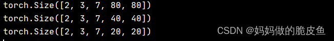
依次为: bachsize, anchors, (obj, class1, class2, x , y ,w, h) , fw, fh
2.2.3 正负样本划分策略
基本步骤:
- 求取标注的bbox的宽高与每层所有anchor的宽高的相互比值,筛选出哪些比值小于4.0(主要是根据模型预测的wh与anchor之间的计算关系而定的)的bbox与anchor的组合;
- 再求取筛选出的bbox与anchor的组合数据的中心坐标相近的2个grid,那么每层中选出的正样本数量就会是第一步中选出样本数量的3倍,正是因为跨网格的匹配策略,导致模型的预测值的的偏移量的范围必须在(-0.5~1.5之间);
代码块详解:
import torch.nn as nn
import torch


# 正样本匹配策略
def convert_data_target(p, targets, device):
    """
    :param device: 设备参数
    :function: 建立target对于计算损失值
    :param p: 就是模型预测值[[2, 3, 52, 80, 7],[2, 3, 26, 40, 7],[2, 3, 13, 20, 7]]
    :param targets: shape(7, 6) 其中7是一个batch的bbox的数量,6表示:(image_id, class, x, y, w, h),bbox来自于哪一个图像,bbox类别,bbox坐标
    :return: 返回转换后的标注数据
    """

    """
    超参数部分:
    """
    nl = 3  # 表示三个检测层
    na = 3  # 每一层的anchors数量
    nt = targets.shape[0]   # 一个batch里所有标注的bbox数量
    anchor_t = 4  # 应该指的是一个长宽比,当标注框与anchor的长宽比小于3.44(最大值为4)时,表示此时的anchor为一个正样本
    anchors = torch.tensor([[10, 13, 16, 30, 33, 23], [30, 61, 62, 45, 59, 119], [116, 90, 156, 198, 373, 326]],device=device).float()
    end_anchors = (anchors / torch.tensor([8, 16, 32],device=device).float().view(3, 1).repeat(1, 6)).view(3, -1, 2)  # shape(3,3,2),不作为模
    """
    第一部分:基础参数部分
    """
    gain = torch.ones(7, device=device)  # shape(7) = [1,1,1,1,1,1,1]

    ai = torch.arange(na, device=device).float().view(na, 1).repeat(1, nt)   # shape(3, 8)
    # cat(torch.Size([3, nt, 6]),torch.Size([3, nt, 1])),将target复制三份用于三个anchor的检测判断
    targets = torch.cat((targets.repeat(na, 1, 1), ai[..., None]), 2)   # (3, 8 , 7),其中7表示:(image_id, class, x, y, w, h, anchor_id)

    g = 0.5  # 偏置,设定相邻grid的筛选范围
    off = torch.tensor([
        [0, 0],
        [1, 0],
        [0, 1],
        [-1, 0],
        [0, -1],   # jk,jm,lk,lm
        ],  device=device).float() * g   # 这里的关键点在于设定4个相邻的grid的区域为0.5的距离,而不是1

    # 存储输出返回值
    tcls, tbox, indices, anch = [], [], [], []

    # 遍历三个输出层
    for i in range(nl):
        """
        target坐标映射到当前层的尺度,假设当前层尺寸为80,则target坐标值乘以80则实现将坐标值映射到了当前层
        """
        anchors = end_anchors[i]  # shape(3,2)    # 获取当前i输出层对应anchors。注意这里的ANCHOR也必须归一化
        shape = p[i].shape                        # 获取模型在i层的推理结果的shape值。
        gain[2:6] = torch.tensor(p[i].shape)[[3, 2, 3, 2]]  # 获取当前层的尺寸[1,1,1,1,1,1,1] = [0, 1, x=80, y=52, x=80, y=52, 6]

        # 实现了将归一化的bbox映射到了当前层的特征图尺寸上
        t = targets * gain     # shape(3, 8 ,7)
        """
        tensor([[
         [ 0.0000,  0.0000, 44.3200, 28.2880, 36.2400, 19.8640,  0.0000],
         [ 0.0000,  1.0000, 44.6400, 28.2880, 35.6000, 20.8520,  0.0000],
         [ 0.0000,  0.0000,  7.8400, 28.6000,  7.2000,  6.7600,  0.0000],
         [ 0.0000,  1.0000, 72.4000, 27.9760,  5.9200,  6.1360,  0.0000],
         [ 0.0000,  1.0000, 16.3200, 13.4160, 20.9600,  7.6960,  0.0000],
         [ 0.0000,  0.0000, 16.8000, 44.5120, 21.2800,  8.3200,  0.0000],
         [ 0.0000,  1.0000, 50.2400,  6.2920, 22.4800,  7.8520,  0.0000],
         [ 0.0000,  0.0000, 51.2000, 48.2040, 23.6800,  5.5640,  0.0000]],

        [[ 0.0000,  0.0000, 44.3200, 28.2880, 36.2400, 19.8640,  1.0000],
         [ 0.0000,  1.0000, 44.6400, 28.2880, 35.6000, 20.8520,  1.0000],
         [ 0.0000,  0.0000,  7.8400, 28.6000,  7.2000,  6.7600,  1.0000],
         [ 0.0000,  1.0000, 72.4000, 27.9760,  5.9200,  6.1360,  1.0000],
         [ 0.0000,  1.0000, 16.3200, 13.4160, 20.9600,  7.6960,  1.0000],
         [ 0.0000,  0.0000, 16.8000, 44.5120, 21.2800,  8.3200,  1.0000],
         [ 0.0000,  1.0000, 50.2400,  6.2920, 22.4800,  7.8520,  1.0000],
         [ 0.0000,  0.0000, 51.2000, 48.2040, 23.6800,  5.5640,  1.0000]],

        [[ 0.0000,  0.0000, 44.3200, 28.2880, 36.2400, 19.8640,  2.0000],
         [ 0.0000,  1.0000, 44.6400, 28.2880, 35.6000, 20.8520,  2.0000],
         [ 0.0000,  0.0000,  7.8400, 28.6000,  7.2000,  6.7600,  2.0000],
         [ 0.0000,  1.0000, 72.4000, 27.9760,  5.9200,  6.1360,  2.0000],
         [ 0.0000,  1.0000, 16.3200, 13.4160, 20.9600,  7.6960,  2.0000],
         [ 0.0000,  0.0000, 16.8000, 44.5120, 21.2800,  8.3200,  2.0000],
         [ 0.0000,  1.0000, 50.2400,  6.2920, 22.4800,  7.8520,  2.0000],
         [ 0.0000,  0.0000, 51.2000, 48.2040, 23.6800,  5.5640,  2.0000]]])
        """

        if nt:   # 如果输入的图像中存在bbox
            """
            1. 查找那些anchor与bbox的长宽比小于anchor_t的anchors
            """
            # 计算bbox与anchor之间的宽高比值
            r = t[..., 4:6] / anchors[:, None]   # torch.Size([3, 8, 2]) / torch.Size([3, 1, 2]) = torch.Size([3, 8, 2])
            # 获取anchor/bbox与bbox/anchor的长宽比中的最大值小于anchor_t的anchors
            j = torch.max(r, 1 / r).max(2)[0] < anchor_t    # shape(3, 8)
            """
            tensor([[False, False, False, False, False, False, False, False],  # 对应anchor0
            [False, False,  True,  True, False, False, False, False],           # 对应anchor1
            [False, False,  True,  True, False, False, False, False]])         # 对应anchor2
            """
            t = t[j]    # 获取当前层i的正样本数据 shape(4, 7) 其中4等于上面true的数量,这样就得到了哪些框需要使用哪个anchor去预测
            """   思考: 由下面的输出可以得出:同一层的多个anchor可以负责预测同一个bbox,一层的anchor不一定能完全匹配所有的bbox。
            tensor([[ 0.0000,  0.0000,  7.8400, 28.6000,  7.2000,  6.7600,  1.0000],   # 最后一列表示该行的bbox由第一层的anchor1预测
                    [ 0.0000,  1.0000, 72.4000, 27.9760,  5.9200,  6.1360,  1.0000],
                    [ 0.0000,  0.0000,  7.8400, 28.6000,  7.2000,  6.7600,  2.0000],
                    [ 0.0000,  1.0000, 72.4000, 27.9760,  5.9200,  6.1360,  2.0000]])
            """

            """
            2. 根据bbox中心点与哪两个grid相邻来筛选正样本,更靠近GT所在的grid则为匹配到的grid
            """
            # 获取真实标框的中心点坐标,注意已经将坐标映射到了当前特征图尺寸shape = (4, 2)
            gxy = t[:, 2:4]

            # 使用当前层的宽高减去中心标注框的中心坐标点shape(4, 2)
            gxi = gain[[2, 3]] - gxy
            """
            tensor([[72.1600, 23.4000],
                    [ 7.6000, 24.0240],
                    [72.1600, 23.4000],
                    [ 7.6000, 24.0240]])
            """
            # (左, 上), gxy > 1排除超过边界的部分shape(1, x), 表示每一个标注框中心左或下也是正样本的bool
            j, k = ((gxy % 1 < g) & (gxy > 1)).T  # 这样做相当于排除了四个角落的可能,前面小于0.5表示靠近左上角,后面大于1表示去除第一行和第一列
            """
            j,k的shape为(4), j表示在左侧,k 表示在上侧: tensor([False, False, False, False]),
            j:(M)   值类型为Bool    如果一个target相对应的值为True,表示该目标中心点所在的格子的左边的格子也对该target进行h回归(后续要计算损失)
            k:(M)   值类型为Bool       表示目标所在格子的 上面的格子
            l:(M)   值类型为Bool       表示目标所在格子的 右边的格子
            m:(M)   值类型为Bool       表示目标所在格子的 下面的格子
            """
            # (右, 下), gxi > 1排除超出边界的部分
            l, m = ((gxi % 1 < g) & (gxi > 1)).T  # 前面小于0.5表示靠近右上角,后面大于1表示去除最后一行和最右一列
            """
            l,m的shape为(4), l表示在右侧,m 表示在下侧: tensor([False, False, False, False]),
            """
            j = torch.stack((torch.ones_like(j), j, k, l, m))   # shape(5, 4), 记录了每一个bbox落在哪一个grid以及与其相邻的2个grid的位置
            """
            # j的value: (5, 4) 4表示当前层的anchor能够匹配的bbox(其中bbox可以重复)
                tensor([[ True,  True,  True,  True],   # 1, 1, 1, 1    中心格
                        [False,  True, False,  True],   # 0, 1, 0, 1    左格
                        [False, False, False, False],   # 0, 0, 0, 0    上格
                        [ True, False,  True, False],   # 1, 0, 1, 0    右格
                        [ True,  True,  True,  True]])  # 1, 1, 1, 1    下格
                        纵向看每列的1的和为3,表示始终只有3个grid,上面第一列表示:第一个bbox使用
            """
            t = t.repeat((5, 1, 1))    # shape(5,4,7)
            t = t[j]                   # shape(12, 7)   原本shape(4,7)表示4个正样本,但是匹配到三个grid后变为12个正样本

            offsets = (torch.zeros_like(gxy)[None] + off[:, None])[j]   # shape(1, 4, 2) + shape(5, 1, 2)[j] = shape(12, 2), 计算得到每个正样本所在grid的偏移量,获取新匹配到grid的真实坐标偏移量
            """
            tensor([[ 0.0000,  0.0000],
                    [ 0.0000,  0.0000],
                    [ 0.0000,  0.0000],
                    [ 0.0000,  0.0000],
                    [ 0.5000,  0.0000],
                    [ 0.5000,  0.0000],
                    [-0.5000,  0.0000],
                    [-0.5000,  0.0000],
                    [ 0.0000, -0.5000],
                    [ 0.0000, -0.5000],
                    [ 0.0000, -0.5000],
                    [ 0.0000, -0.5000]])
            """

        else:   # 相当于输入的图片中没有bbox时如何处理
            t = targets[0]   # 获取得到第一个bbox[1, 6]
            offsets = 0  # 设置偏置等于0

        """
        计算匹配到的grid左上坐标点
        """
        # (image, class), grid xy, grid wh, anchors
        bc, gxy, gwh, a = t.chunk(4, 1)
        """
        bc = shape(12, 2)   gxy = shape(12, 2)  a = shape(12)
        """
        # 12个正样本对应的anchors, image_id, class_id
        a, (b, c) = a.long().view(-1), bc.long().T

        gij = (gxy - offsets).long()   # 计算所有正样本所在grid的左上角坐标
        """
        tensor([[ 7, 28],
        [72, 27],
        [ 7, 28],
        [72, 27],
        [71, 27],
        [71, 27],
        [ 8, 28],
        [ 8, 28],
        [ 7, 29],
        [72, 28],
        [ 7, 29],
        [72, 28]])
        """
        # grid 的索引
        gi, gj = gij.T    # x, y
        """
        clamp(a, b, x) = a         x ≤ a
                       = x         a ≤ x ≤ b
                       = b         x ≥ b
        """
        # image_id, anchor_index, grid(格子左上坐标(gj表示高索引,gi表示宽索引))
        images_index = list(set(b.numpy()))
        tem_b = b.numpy()
        for img_index in range(len(tem_b)):
            index_tem = images_index.index(b[img_index])
            tem_b[img_index] = index_tem
        b = torch.tensor(tem_b)

        indices.append((b, a, gj.clamp_(0, shape[2] - 1), gi.clamp_(0, shape[3] - 1)))  #
        tbox.append(torch.cat((gxy - gij, gwh), 1))  # box
        anch.append(anchors[a])  # anchors

        tcls.append(c)  # class
    # 返回3个输出层使用anchor,grid匹配到的所有的正样本bbox
    return tcls, tbox, indices, anch
2.2.4 使用正样本划分后的结果计算损失函数值
# 下面所有函数与convert_data_target同在一个.py文件

# 用于计算p_box与bbox之间的iou,其中box1=shape(1,4); box2 = shape(n,4)
def bbox_iou(box1, box2, xywh=True,GIoU=False,DIoU=False,CIoU=False,eps=1e-7):
    """
    :6.0使用的是CIOU损失
    :param box1: 预测框之一
    :param box2: 正样本标注框
    :param xywh: 指定box输入的格式,如果为True就表示输入xywh,不是就表示输入的是左上角与右下角坐标
    :param GIOU: 下面是三种计算交并比的实现方法
    :param DIOU:
    :param CIou:
    :param eps:
    :return: 返回shape(n)返回的是每一个预测值与所有真实框之间的交并比
    """
    if xywh:  # transform from xywh to xyxy
        (x1, y1, w1, h1), (x2, y2, w2, h2) = box1.chunk(4, -1), box2.chunk(4, -1)
        w1_, h1_, w2_, h2_ = w1 / 2, h1 / 2, w2 / 2, h2 / 2
        b1_x1, b1_x2, b1_y1, b1_y2 = x1 - w1_, x1 + w1_, y1 - h1_, y1 + h1_
        b2_x1, b2_x2, b2_y1, b2_y2 = x2 - w2_, x2 + w2_, y2 - h2_, y2 + h2_
    else:  # x1, y1, x2, y2 = box1
        b1_x1, b1_y1, b1_x2, b1_y2 = box1.chunk(4, -1)
        b2_x1, b2_y1, b2_x2, b2_y2 = box2.chunk(4, -1)
        w1, h1 = b1_x2 - b1_x1, (b1_y2 - b1_y1).clamp(eps)   # 保证所有预测的box的宽高不为0,相当于平滑标签处理
        w2, h2 = b2_x2 - b2_x1, (b2_y2 - b2_y1).clamp(eps)

    # 计算交叉面积
    inter = (b1_x2.minimum(b2_x2) - b1_x1.maximum(b2_x1)).clamp(0) * \
            (b1_y2.minimum(b2_y2) - b1_y1.maximum(b2_y1)).clamp(0)

    # 计算并集面积
    union = w1 * h1 + w2 * h2 - inter + eps     # 也进行的防止为0的措施

    # 计算交并比
    iou = inter / union
    if CIoU or DIoU or GIoU:
        cw = b1_x2.maximum(b2_x2) - b1_x1.minimum(b2_x1)  # convex (smallest enclosing box) width
        ch = b1_y2.maximum(b2_y2) - b1_y1.minimum(b2_y1)  # convex height
        if CIoU or DIoU:  # Distance or Complete IoU
            c2 = cw ** 2 + ch ** 2 + eps  # convex diagonal squared
            rho2 = ((b2_x1 + b2_x2 - b1_x1 - b1_x2) ** 2 + (b2_y1 + b2_y2 - b1_y1 - b1_y2) ** 2) / 4  # center dist ** 2
            if CIoU:
                v = (4 / math.pi ** 2) * (torch.atan(w2 / h2) - torch.atan(w1 / h1)).pow(2)
                with torch.no_grad():
                    alpha = v / (v - iou + (1 + eps))
                return iou - (rho2 / c2 + v * alpha)  # CIoU
            return iou - rho2 / c2  # DIoU
        c_area = cw * ch + eps  # convex area
        return iou - (c_area - union) / c_area
    return iou

# 类别标签平滑处理
def smooth_BCE(eps=0.1):
    # return positive, negative label smoothing BCE targets
    return 1.0 - 0.5 * eps, 0.5 * eps

# FocalLoss损失函数的定义,可以更换其他均衡化样本的方法
class FocalLoss(nn.Module):
    def __init__(self, loss_fcn, gamma=1.5, alpha=0.25):
        super().__init__()
        self.loss_fcn = loss_fcn  # must be nn.BCEWithLogitsLoss()
        self.gamma = gamma
        self.alpha = alpha
        self.reduction = loss_fcn.reduction
        self.loss_fcn.reduction = 'none'  # required to apply FL to each element

    def forward(self, pred,  true):
        loss = self.loss_fcn(pred, true)
        pred_prob = torch.sigmoid(pred)  # prob from logits
        p_t = true * pred_prob + (1 - true) * (1 - pred_prob)
        alpha_factor = true * self.alpha + (1 - true) * (1 - self.alpha)
        modulating_factor = (1.0 - p_t) ** self.gamma
        loss *= alpha_factor * modulating_factor

        if self.reduction == 'mean':    # 反向传播的反馈量是均值还是和
            return loss.mean()
        elif self.reduction == 'sum':
            return loss.sum()
        else:  # 'none'
            return loss

# 用于计算yolo的损失函数值
def computer_yolo_loss(p, targets, device):
    """
    基础参数设置部分
    """
    sort_obj_iou = False
    na = 3    # anchor的数量
    nc = 2    # 类别数量
    nl = 3    # 指定模型输出层数
    gr = 0.8  # 用于将iou的值限制在0~1的范围,并作为置信度值
    bs = p[0].shape[0]   # batch size
    balance = {

    3: [4.0, 1.0, 0.4]}.get(nl, [4.0, 1.0, 0.25, 0.06, 0.02])  # 默认是输出3层每层损失对应权重是(4,1,0.4)当大于3时取后面的
    ssi = list([8, 16, 32]).index(16)  # 下采样16倍的索引值为1
    auto_balance = True
    # 指定anchors
    anchor_values = torch.tensor([[10, 13, 16, 30, 33, 23], [30, 61, 62, 45, 59, 119], [116, 90, 156, 198, 373, 326]],device=device).float()
    anchors = (anchor_values / torch.tensor([8, 16, 32], device=device).float().view(3, 1).repeat(1, 6)).view(3, -1,2)

    # 定义类别损失函数和置信度损失函数,都是用log损失函数
    BCE_cls = nn.BCEWithLogitsLoss(pos_weight=torch.tensor([1.0], device=device))
    BCE_obj = nn.BCEWithLogitsLoss(pos_weight=torch.tensor([1.0], device=device))

    # 类别标签平滑处理
    cp, cn = smooth_BCE(eps=0.1)  # positive, negative BCE targets,使用默认值

    # focal loss
    g = 0.0  # focal loss gamma
    if g > 0:
        BCE_cls, BCE_obj = FocalLoss(BCE_cls, g), FocalLoss(BCE_obj, g)
    """
    实现yolo损失的计算
    """
    # 定义三种损失变量,用于存储三个部分的损失值
    lcls = torch.zeros(1, device=device)  # class loss
    lbox = torch.zeros(1, device=device)  # box loss
    lobj = torch.zeros(1, device=device)  # object loss

    # 获取正样本的相关数据(下面函数build_targets函数中pre参数只是起提供shape的作用)
    tcls, tbox, indices, anchors = convert_data_target(p, targets, device)
    """
     # tcls:[shape(12), shape(42), shape(48)] 存储的是每层的所有正样本的类别
     # tbox:[shape(12, 4), shape(42,4), shape(48, 4)] 存储的是每层所有正样本的bbox的 bia_xy, wh值
     # indices:[(12,4),(42,4),(48,4)]  image_id, anchor_index, grid_y,grid_x
     # anchors:[shape(12, 2),shape(42,2),shape(48, 2)] 存储的是每层所有正样本使用的anchor的大小
    """
    # 计算损失值
    for i, pi in enumerate(p):   # 输出层索引, 每层的预测值
        b, a, gj, gi = indices[i]  # 图像索引, anchor索引, grid的y的索引, grid的x的索引
        tobj = torch.zeros(pi.shape[:4], dtype=pi.dtype, device=device)  # target obj,shape=(batch_size,3,h,w )

        n = b.shape[0]  # number of targets
        if n:
            # 获取预测的xy偏置以及wh和类别,等号右边的shape=(N,nc+5),其中N等于正样本数量,且位置是一一对应关系
            pxy, pwh, _, pcls = pi[b, a, gj, gi].tensor_split((2, 4, 5), dim=1)

            # 回归计算,定位损失
            pxy = pxy.sigmoid()*2 - 0.5    # 约束取值范围到了(-0.5~1.5,为了扩大正样本数量,对应于跨网格策略)
            pwh = (pwh.sigmoid()*2)**2*anchors[i]  # 约束预测的wh只能是由anchors在4倍的变化范围内

            # 获取得到坐标变换后的预测框
            pbox = torch.cat((pxy, pwh), 1)  # shape(batch, N, 4)

            # 计算交并比
            iou = bbox_iou(pbox, tbox[i], CIoU=True).squeeze()  # shape(N)

            # 获取iou损失, 交并比越大损失值越小
            lbox += (1.0 - iou).mean()

            # 计算置信度
            iou = iou.detach().clamp(0).type(tobj.dtype)  # 将iou从计算图中分离,不存储梯度

            if sort_obj_iou:
                j = iou.argsort()    # 返回的是iou从小到大排序的索引值
                b, a, gj, gi, iou = b[j], a[j], gj[j], gi[j], iou[j]  # 按照iou从小到大对图像\anchor\grid坐标的索引重新排序
            if gr < 1:
                iou = (1.0 - gr) + gr * iou  # 强制iou的取值范围为(0~1)之间
            # tobj = shape=(batch_size,3,h,w ), 下面等式左侧shape(N, 1)
            tobj[b, a, gj, gi] = iou  # 使用iou的值作为正样本grid处的置信度,非正样本grid直接设置为0

            # Classification
            if nc > 1:  # cls loss (only if multiple classes)
                t = torch.full_like(pcls, cn, device=device)  # targets
                t[range(n), tcls[i]] = cp
                lcls += BCE_cls(pcls, t)  # BCE

        obji = BCE_obj(pi[..., 4], tobj)

        # 对每层的计算损失使用权重平衡,主要用于扩大小目标的反馈量
        lobj += obji * balance[i]  # obj loss
        if auto_balance:
            balance[i] = balance[i] * 0.9999 + 0.0001 / obji.detach().item()

    # 对类别、置信度、定位损失设置不同的权重值
    if auto_balance:
        balance = [x / balance[ssi] for x in balance]

    lbox *= 0.05          # self.hyp['box']  定位损失权重
    lobj *= 0.7           # self.hyp['obj']  置信度损失
    lcls *= 0.3           # self.hyp['cls']  分类损失

    # 返回整个batch的损失值和, 以及整个batch中三个分量损失值
    return (lbox + lobj + lcls) * bs, torch.cat((lbox, lobj, lcls)).detach()
前向测试展示
import ComFunction
import torch
import Detection
import GroundDataTolabel
import cv2
import sample_np_split

if __name__ == '__main__':
    device = torch.device('cuda' if torch.cuda.is_available() else 'cpu')
    model = ComFunction.BackOne(2, 1).to(device)
    # summary(model, (416, 640), -1)
    data = torch.rand((1, 3, 416, 640)).to(device)
    img = cv2.imread("C:/Users/620H/Desktop/save_img/1.jpg", cv2.COLOR_BGR2RGB)
    img_tensor = (torch.from_numpy(img).to(device)[None].permute(0, 3, 1, 2)).float()

	# 该targets符合yolo格式,(图像索引,类别索引,x,y,w,h)
    targets = torch.tensor([[0, 0 ,0.554 ,0.544, 0.453, 0.382],
                            [0, 1 ,0.558 ,0.544, 0.445, 0.401 ],
                            [0, 0 ,0.098, 0.550, 0.090 ,0.130],
                            [0, 1 ,0.905 ,0.538 ,0.074 ,0.118],
                            [0, 1 ,0.204 ,0.258 ,0.262 ,0.148],
                            [0, 0 ,0.210, 0.856 ,0.266, 0.160],
                            [0, 1 ,0.628 ,0.121 ,0.281, 0.151],
                            [0, 0 ,0.640, 0.927 ,0.296 ,0.107]], device=device).float()
    pre_y = model(img_tensor)  # 模型的前向计算

    # 调用损失计算函数
    a, b = sample_np_split.computer_yolo_loss(pre_y, targets, device)
    print("all_loss:"a)
    print("brance_loss:", b)
"""
输出结果为:
all_loss: tensor([3.4023], grad_fn=<MulBackward0>)
brance_loss: tensor([0.1057, 2.6722, 0.6243])
"""
2.2.5 模型训练的基本过程
2.2.5.1 构建数据管道
# 用于创建yolo需要的数据管道
import pandas as pd
import torch
from torch.utils.data import Dataset
from torchvision import datasets
import os
import cv2

class MyDataset(Dataset):
    def __init__(self, image_dir, label_dir, transform=None):
        """
        Args:
            image_dir: path to image directory.
            label_dir: path to label directory
            transform: optional transform to be applied on a sample.
        """
        self.label_dir = label_dir
        self.image_dir = image_dir

        self.image_list = os.listdir(image_dir)
        self.label_list = os.listdir(label_dir)

        self.transform = transform

    def __getitem__(self, index):
        """
        Args:
            index: the index of item
        Returns:
            image and its targets:tensor([image_id, class_id, x, y, w, h])
        """
        image_name = os.path.join(self.image_dir, self.image_list[index])
        image = cv2.imread(image_name, cv2.COLOR_BGR2RGB)

        image_id = int(self.image_list[index].split(".")[0])

        # 读取label
        label_name = str(image_id) + ".txt"
        label_path = os.path.join(self.label_dir, label_name)

        # 获取图像对应的标注数据[[0.553646, 0.545417, 0.453125, 0.3975, 15.0],[0.553646, 0.545417, 0.453125, 0.3975, 15.0]]
        per_labels_list = []
        with open(label_path, "r", encoding='utf-8') as f_label:
            all_labels = f_label.readlines()
            for per_label in all_labels:
                per_label = per_label.strip("\n")
                split_label = per_label.split()
                a = [float(tem_i) for tem_i in split_label]
                tem_list = [image_id, a[-1], a[0], a[1], a[2],a[3]]
                # tem_list.extend([int(split_label[4:])

                print(tem_list)
                per_labels_list.append(tem_list)
        f_label.close()
        targets = torch.tensor(per_labels_list)

        if self.transform is not None:
            image = self.transform(image)
        return image, targets

    def __len__(self):
        return len(self.image_list)
数据管道测试:
import ComFunction
import torch
import Detection
import GroundDataTolabel
import cv2
import sample_np_split
import InitializeModle
from torch.utils.data import DataLoader
import SetDataLoader
from torchvision import datasets
if __name__ == '__main__':
device = torch.device('cuda' if torch.cuda.is_available() else 'cpu')
# dataloader测试
image_file = "C:/Users/620H/Desktop/save_img"
yolo_label_file = "C:/Users/620H/Desktop/save_label"
import os
train_data = SetDataLoader.MyDataset(image_file, yolo_label_file)
train_loader = torch.utils.data.DataLoader(train_data, batch_size=2, num_workers=1, shuffle=True,
drop_last=True)
import matplotlib.pyplot as plt
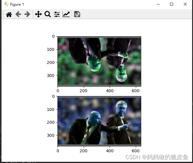
images, labels = next(iter(train_loader))
plt.figure()
plt.subplot(2, 1, 1)
plt.imshow(images[0])
plt.subplot(2, 1, 2)
plt.imshow(images[1])
plt.show()
"""
image_shape: label_shape, 必须保证所有图像的尺寸一致
图像尺寸: torch.Size([3, 384, 640, 3]) 标签: torch.Size([3, 4, 6])
"""
2.2.5.1 构建训练过程
import ComFunction
import torch
import torch.nn as nn
import Detection
import GroundDataTolabel
import cv2
import sample_np_split
from torch.optim import lr_scheduler
import InitializeModle
from torch.utils.data import DataLoader
import SetDataLoader
from torchvision import datasets
if __name__ == '__main__':
device = torch.device('cuda' if torch.cuda.is_available() else 'cpu')
model = ComFunction.BackOne(5, 2).to(device) # 定义模型
# 模型参数初始化
InitializeModle.initialize_weights(model)
# 加载数据,这里只加载训练数据
image_file = "C:/Users/620H/Desktop/save_img"
yolo_label_file = "C:/Users/620H/Desktop/save_label"
# 构建训练数据的管道
train_data = SetDataLoader.MyDataset(image_file, yolo_label_file)
train_loader = torch.utils.data.DataLoader(train_data, batch_size=2, num_workers=1, shuffle=True, drop_last=True)
# 构建优化器
g = [], [], [] # 将不同层的参数进行分离,以方便使用不同的优化策略去更新这些模型参数
bn = tuple(v for k, v in nn.__dict__.items() if 'Norm' in k) # normalization layers, i.e. BatchNorm2d()
for v in model.modules():
for p_name, p in v.named_parameters(recurse=False):
if p_name == 'bias': # bias (no decay)
g[2].append(p)
elif p_name == 'weight' and isinstance(v, bn): # weight (no decay)
g[1].append(p)
else:
g[0].append(p) # weight (with decay)
optimizer = torch.optim.Adam(g[2], lr=0.01, betas=(0.001, 0.999)) # 使用'Adam'优化器,只对卷积权重进行优化
# 定义训练批次
epochs = 300
# 定义学习率衰减策略
lf = lambda x: (1 - x / epochs) * (1.0 - 0.1) + 0.1 # linear
scheduler = lr_scheduler.LambdaLR(optimizer, lr_lambda=lf) # plot_lr_scheduler(optimizer, scheduler, epochs)
nb = len(train_loader) # 获取所有图像可以检索的批次数量
for epoch in range(epochs):
model.train()
m_loss = torch.zeros(3, device=device)
optimizer.zero_grad()
for i, (images, labels) in enumerate(train_loader):
ni = i + nb * epoch
# 将图像转换为tensor并进行归一化处理
images = (torch.as_tensor(images.data, device=device).float() / 255).permute(0, 3, 1, 2)
# 前向运算
pre_result = model(images)
shape = labels.size()
targets = labels.view(-1, shape[2]) # 需要将所有batch的bbox全部reshape到2维
all_loss, item_loss = sample_np_split.computer_yolo_loss(pre_result, targets, device)
# 反向传播
all_loss.backward()
optimizer.step()
optimizer.zero_grad()
m_loss = (m_loss * i + item_loss) / (i + 1)
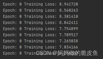
print('Epoch: {} Training Loss: {:.6f}'.format(epoch, all_loss.item()))
lr = [x['lr'] for x in optimizer.param_groups]
scheduler.step()
print('Epoch: {} /tTraining Loss: {:.6f}'.format(epoch, m_loss[1].item()))
# 模型权重初始化函数
import torch
import torch.nn as nn

def initialize_weights(self):
	for m in self.modules():
		# 判断是否属于Conv2d
		if isinstance(m, nn.Conv2d):
			torch.nn.init.xavier_normal_(m.weight.data)
			# 判断是否有偏置
			if m.bias is not None:
				torch.nn.init.constant_(m.bias.data,0.3)
		elif isinstance(m, nn.Linear):
			torch.nn.init.normal_(m.weight.data, 0.1)
			if m.bias is not None:
				torch.nn.init.zeros_(m.bias.data)
		elif isinstance(m, nn.BatchNorm2d):
			m.weight.data.fill_(1)
损失值逐渐收敛:
2.2.5.2 可视化模型训练过程(方便于记录整个模型训练的过程,以及参数调优。)
pip install tensorboardX
基本流程:
from tensorboardX import SummaryWriter
# 也可以使用pytorch自带的tensorboard
# from torch.utils.tensorboard import SummaryWriter
writer = SummaryWriter('./runs')   # 指定监测数据的存储目录

writer.add_    # 用于添加具体的数据类型
writer.close()
浏览器端启动tensorboard
# 命令行启动命令/path/to/logs/为指定的监测数据存储目录,启动时/path/to/logs/最好是绝对路劲
tensorboard --logdir=/path/to/logs/
- 可视化网络结构
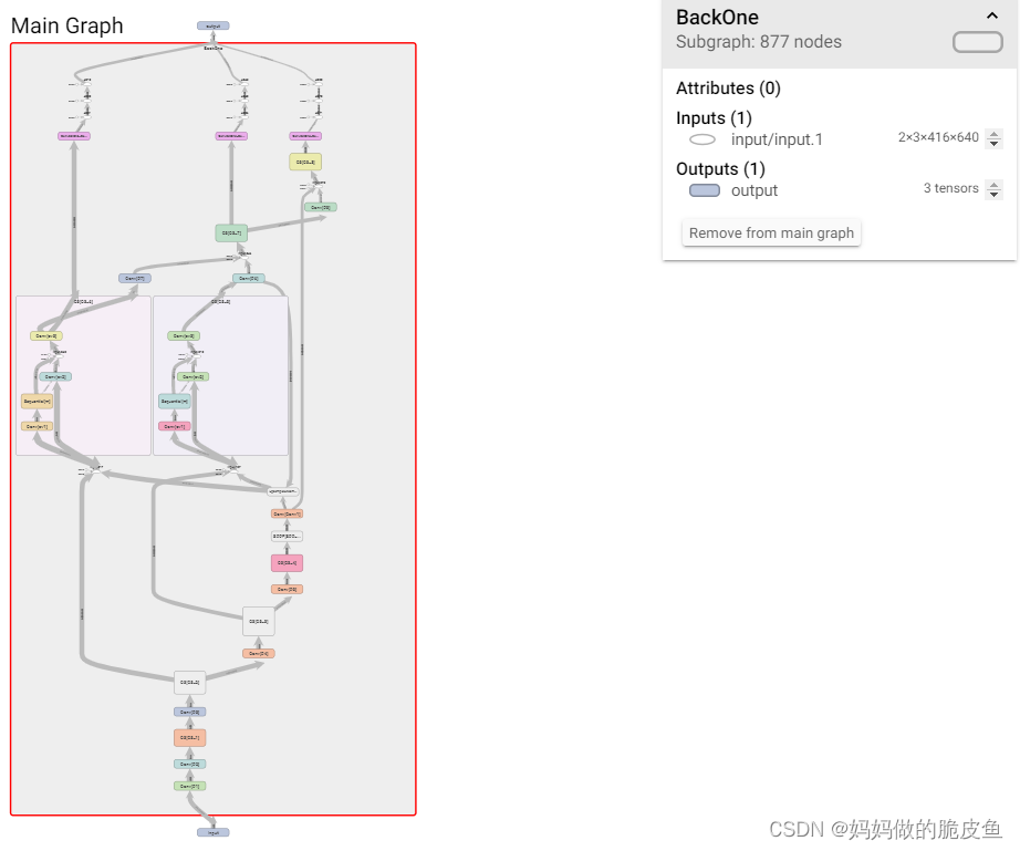
- 可视化图像数据
# 仅查看一张图片
writer = SummaryWriter('./pytorch_tb')
writer.add_image('images', image)
writer.close()
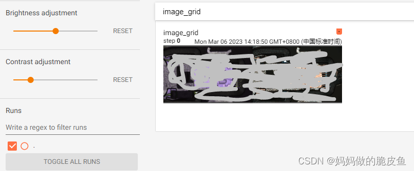
# 将多张图片拼接成一张图片,中间用黑色网格分割
# create grid of images
writer = SummaryWriter('./pytorch_tb')
img_grid = torchvision.utils.make_grid(images)
writer.add_image('image_grid', img_grid)
writer.close()
# 将多张图片直接写入
writer = SummaryWriter('./pytorch_tb')
writer.add_images("images",images,global_step = 0)
writer.close()
# 测试代码
 for i, (images, labels) in enumerate(train_loader):
            ni = i + nb * epoch

            # 将图像显示到tensorboard,可以使用以上三种方法进行替换
            if i == 0:
                writer = SummaryWriter('./images')
                writer.add_images('image_grid', images.permute(0,3,1,2))
                writer.close()
		    if i == 1:              #  将多张图显示到一张画布上
                writer = SummaryWriter('./images')
                img_grid = torchvision.utils.make_grid(images.permute(0, 3, 1, 2))
                writer.add_image('image_grid', img_grid)
                writer.close()

            # 将图像转换为tensor并进行归一化处理
            images = (torch.as_tensor(images.data, device=device).float() / 255).permute(0, 3, 1, 2)

            # 前向运算
            pre_result = model(images)
            shape = labels.size()
            targets = labels.view(-1, shape[2])  # 需要将所有batch的bbox全部reshape到2维
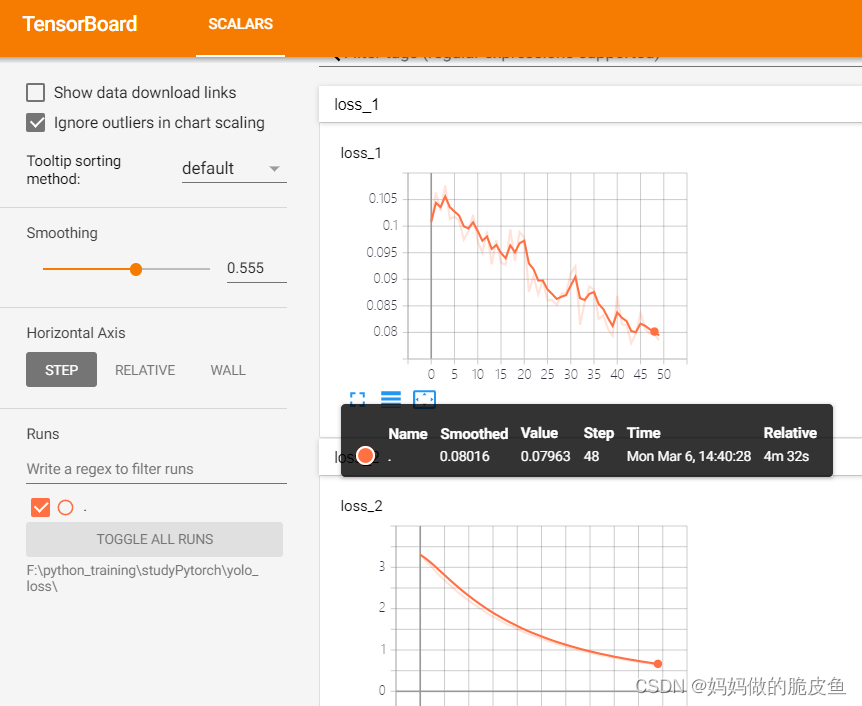
- 可视化连续数据比如损失值
# 显示在不同的画布上
 writer = SummaryWriter('./yolo_loss')  # 创建监视目录
 for epoch in range(1):
        model.train()

        m_loss = torch.zeros(3, device=device)
        optimizer.zero_grad()

        for i, (images, labels) in enumerate(train_loader):
            m_loss = (m_loss * i + item_loss) / (i + 1)
            print('Epoch: {} Training Loss: {:.6f}'.format(epoch, all_loss.item()))
			writer.add_scalar("loss_1", m_loss[0].item(), i) #日志中记录x在第step i 的值   写入损失值
			writer.add_scalar("loss_2", m_loss[1].item(), i) #日志中记录y在第step i 的值
        lr = [x['lr'] for x in optimizer.param_groups]
        scheduler.step()
        print('Epoch: {} /tTraining Loss: {:.6f}'.format(epoch, m_loss[1].item()))
writer.close()
只是用于测试,没有进行整个模型的训练
- 可视化参数分布
# 显示在相同的画布上
writer1 = SummaryWriter('./pytorch_tb/x')  # 创建两个不同的子集目录,但是父目录相同
writer2 = SummaryWriter('./pytorch_tb/y')
for i in range(500):
    x = i
    y = x*2
    writer1.add_scalar("same", x, i) #日志中记录x在第step i 的值
    writer2.add_scalar("same", y, i) #日志中记录y在第step i 的值
writer1.close()
writer2.close()
2.2.5.3 模型保存与读取
- pytorch支持的模型保存的常见格式:.pkl, .pt, .pth
- 模型保存内容分为网络结构和模型参数两部分内容:模型参数是以模型层名称为键以权重向量为值的一个字典。
- 保存模型有两个选择:保存模型结构与权重,或只保存权重。
单卡保存与单卡调用的基本流程:
import os
import torch
from torchvision import models

os.environ['CUDA_VISIBLE_DEVICES'] = '0'   #这里替换成希望使用的GPU编号
model = models.resnet152(pretrained=True)
model.cuda()

# step1: 设置保存路劲以及保存格式
save_dir = 'resnet152.pt'

# step2: 保存模型到指定的路劲
torch.save(model, save_dir)

# step3: 加载模型
loaded_model = torch.load(save_dir)

# step4: 将模型迁移到指定的设备
# device = torch.device('cuda' if torch.cuda.is_available() else 'cpu')
loaded_model.cuda()   # 也可以使用.to(device)

"""
只保存参数,不保存网络结构
"""
torch.save(model.state_dict(), save_dir)    # 选择只保存权重
loaded_model = models.resnet152()   #注意这里需要对模型结构有定义
loaded_model.load_state_dict(torch.load(save_dir))  # 将参数赋值给模型结构
loaded_model.cuda()
2.2.5.3 模型部署与调用过程(并使用yolo_v5模型进行部署测试验证)
本小节参考地址1
onnx官网教程
onnx runtime官网
1. 导出为ONNX格式,并使用ONNX RUN TIME 去实现推理过程(推荐该方法)
onnx runtime基本特点:
- 提高各种ML模型的推理性能;
- 在不同的硬件和操作系统上运行;
- 在python中训练,但部署到c#/c++/java应用程序中
- 可以使用在不同框架中创建的模型训练和执行推理
基本流程:
- 获取模型-----pytorch的.pkl, .pt, .pth----->ONNX格式(执行这一步时,要注意那些算子是ONNX支持的,否则可能会失败,也可以根据官网自定义算子);
- 用ONNX RUNTIME去运行加载的ONNX模型;
- 使用硬件加速器或各种配置实现模型性能的优化,一般情况使用ONNX RUNTIME执行推理的性能要好于原始模型所在的框架;
# 流程1---获取/加载模型,并导出为onnx
resnet50 = models.resnet50(pretrained=True)

# 导出模型为ONNX
image_height = 224
image_width = 224
x = torch.randn(1, 3, image_height, image_width, requires_grad=True)
torch_out = resnet50(x)
torch.onnx.export(resnet50,                     # model being run
                  x,                            # model input (or a tuple for multiple inputs)
                  "resnet50.onnx",              # 保存onnx模型的路径
                  export_params=True,           # 如果模型是预训练好的就为True
                  opset_version=12,             # 使用的ONNX的版本号
                  do_constant_folding=True,     # 是否执行常量折叠优化
                  input_names = ['input'],      # 模型输入的名称
                  output_names = ['output'],    # 模型输出的名称
                  dynamic_axes={

    'input' : {

    0 : 'batch_size'},
                                'output' : {

    0 : 'batch_size'}})
# 流程2: 使用ONNX Runtime实现模型推理(python)
import onnxruntime
from onnx import numpy_helper
import time

# 1. 获取ONNX Runtime 推理器
session_fp32 = onnxruntime.InferenceSession("resnet50.onnx", providers=['CPUExecutionProvider'])    # 使用CPU,选用该方法
# session_fp32 = onnxruntime.InferenceSession("resnet50.onnx", providers=['CUDAExecutionProvider'])   # 使用GPU
# session_fp32 = onnxruntime.InferenceSession("resnet50.onnx", providers=['OpenVINOExecutionProvider'])   # 使用OPENVINO

# 2. 执行推理
# 构建字典的输入数据,字典的key需要与我们构建onnx模型时的input_names相同
# 输入的input_img 也需要改变为ndarray格式
ort_inputs = {

    'input': input_img}
# 我们更建议使用下面这种方法,因为避免了手动输入key
# ort_inputs = {ort_session.get_inputs()[0].name:input_img}

# run是进行模型的推理,第一个参数为输出张量名的列表,一般情况可以设置为None
# 第二个参数为构建的输入值的字典
# 由于返回的结果被列表嵌套,因此我们需要进行[0]的索引
ort_output = ort_session.run(None,ort_inputs)[0]
c++使用onnx runtime实现onnx模型的推理案例yolov5: https://github.com/DefTruth/lite.ai.toolkit/tree/main/lite/ort/cv
开源项目大览: https://zhuanlan.zhihu.com/p/414317269
2. 导出为torchscript格式,然后使用libtorch实现c++推理
pytorch官方文档有详细说明
2.2.5.4 训练优化策略
训练优化策略参考地址: https://blog.csdn.net/CharmsLUO/article/details/123577851
2.3 以开源PCB数据为例实现yolov5从训练到模型部署的全过程
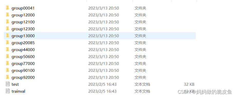
2.3.1 PCB数据标准化为YOLOV5的输入数据格式
PCB Dataset开源数据集,这里我就不放链接了,自己有需要github搜索。
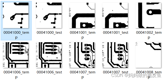
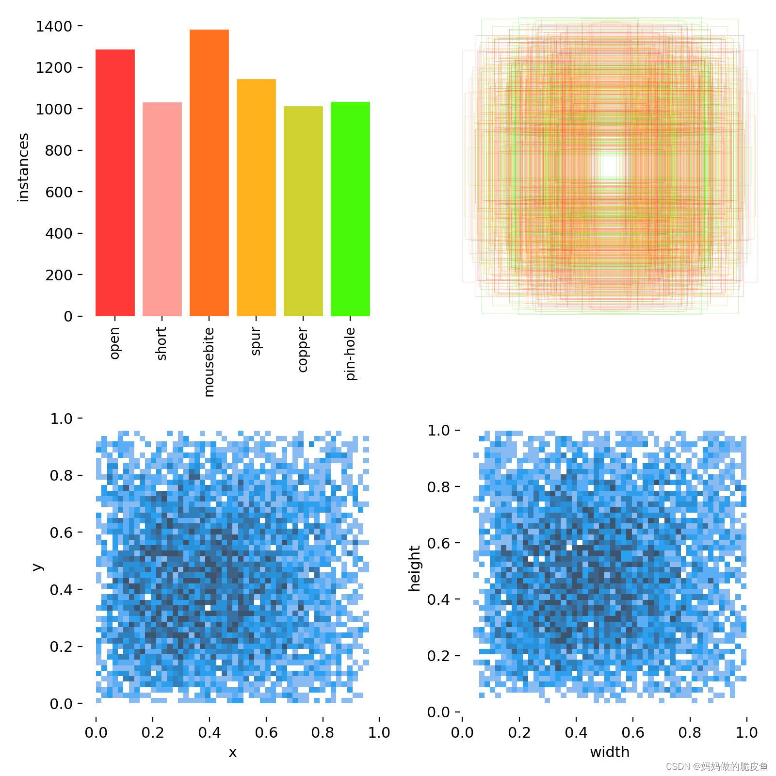
数据类别:
names:
  0: open
  1: short
  2: mousebite
  3: spur
  4: copper
  5: pin-hole
下图反映了该数据集各类缺陷对象的数量,以及gt框在图像上的分布情况、gt框的长宽和中心分布。
使用下面代码可以将上面PCB数据转换为yolo对应的数据集类型(yolo需要的数据结构可以参考上面的第一章的内容):
import cv2
import os
image_list = []
image_annotations = []
# 主要用于显示样本和标框
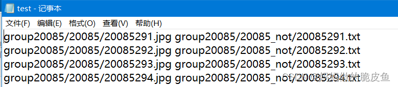
def disp_samples():
with open("PCBData/trainval.txt", "r") as file:
line_text = file.readlines()
for per_path in line_text:
per_path_list = per_path.strip("/n").split()
image_list.append("E:/deepleaning/self_yolov5/PCBData/" + per_path_list[0].split(".")[0] + "_test.jpg")
image_annotations.append("E:/deepleaning/self_yolov5/PCBData/" + per_path_list[1])
file.close()
for i in range(len(image_list)):
image = cv2.imread(image_list[i], cv2.COLOR_GRAY2RGB)
cl = len(image.shape)
if cl == 2:
image = cv2.cvtColor(image, cv2.COLOR_GRAY2RGB)
with open(image_annotations[i], "r") as file:
boxes = file.readlines()
for per_box in boxes:
per_box = per_box.strip("/n")
box_value = per_box.split()
cv2.rectangle(image, (int(box_value[0]), int(box_value[1])), (int(box_value[2]), int(box_value[3])), (0, 0, 255))
# cv2.imshow("t1", image)
# cv2.waitKey(2000)
file.close()
def all_data_augmentation(save_img_file, label_save_file):
"""
:param save_img_file: "E:/deepleaning/self_yolov5/images/
:param label_save_file: "E:/deepleaning/self_yolov5/labels/
"""
files_image = image_list # 读取给定的图像存储文件夹
files_label = image_annotations # 读取存储给定的标注数据存储文件夹
len1, len2 = int(len(files_image)), int(len(files_label))
if len1 == len2:
for i in range(len1):
# 获取得到图像完整路径
image_path = image_list[i]
# 获取得到图像对应标签的完整路劲
label_path = image_annotations[i]
# 获取图像
image1 = cv2.imread(image_path)
cl = len(image1.shape)
if cl == 2:
image1 = cv2.cvtColor(image1, cv2.COLOR_GRAY2RGB)
# 获取图像对应的标注数据[[0.553646, 0.545417, 0.453125, 0.3975, 15.0],[0.553646, 0.545417, 0.453125, 0.3975, 15.0]]
per_labels_list = []
with open(label_path, "r", encoding='utf-8') as f_label:
all_labels = f_label.readlines()
for per_label in all_labels:
per_label = per_label.strip("\n")
split_label = per_label.split()
tem_list = [int(float(split_label[-1])-1)]
for tem_i in split_label[:4]:
tem_list.append(float(tem_i) / 640)
per_labels_list.append(tem_list)
f_label.close()
# 获取图像存储名,并保存
image_name = image_path.split("/")[-1].split("_")[0]
new_img_path = save_img_file + str(image_name) + ".jpg"
cv2.imwrite(new_img_path, image1)
# 获取保存标注的文件名和路径
new_label_name = str(image_name) + ".txt"
new_label_path = label_save_file + new_label_name
f = open(new_label_path, "w")
len_box = len(per_labels_list)
for i in range(len_box):
per_box = per_labels_list[i]
for j in range(len(per_box)):
per_value = per_box[j]
if j == 0:
print(per_value)
per_value = format(per_value, '.3f') # 只保留三位小数点
f.write(str(per_value))
if j < len(per_box) - 1:
f.write(" ")
if i < len_box - 1: # 保证在写入最后一行数据结束后不再添加换行符
f.write("\n")
f.close()
return
else:
return
if __name__ == '__main__':
disp_samples()
save_img_file = "E:/deepleaning/self_yolov5/images/"
label_save_file = "E:/deepleaning/self_yolov5/labels/"
all_data_augmentation(save_img_file, label_save_file)
2.3.2 超参数和基本训练配置参数的设置
# 超参数
lr0: 0.01  # 初始学习率 (SGD=1E-2, Adam=1E-3)
lrf: 0.01  # 循环学习率 (lr0 * lrf)
momentum: 0.937  # SGD momentum/Adam beta1 学习率动量
weight_decay: 0.0005  # 权重衰减系数
warmup_epochs: 3.0  # 预热学习 (fractions ok)
warmup_momentum: 0.8  # 预热学习动量
warmup_bias_lr: 0.1  # 预热初始学习率
box: 0.05  # iou损失系数
cls: 0.5  # cls损失系数
cls_pw: 1.0  # cls BCELoss正样本权重
obj: 1.0  # 有无物体系数(scale with pixels)
obj_pw: 1.0  # 有无物体BCELoss正样本权重
iou_t: 0.20  # IoU训练时的阈值
anchor_t: 4.0  # anchor的长宽比(长:宽 = 4:1)
# anchors: 3  # 每个输出层的anchors数量(0 to ignore)
#以下系数是数据增强系数,包括颜色空间和图片空间
fl_gamma: 0.0  # focal loss gamma (efficientDet default gamma=1.5)

# 下面使图像增强相关参数
hsv_h: 0.015  # 色调 (fraction)
hsv_s: 0.7  # 饱和度 (fraction)
hsv_v: 0.4  # 亮度 (fraction)
degrees: 0.0  # 旋转角度 (+/- deg)
translate: 0.1  # 平移(+/- fraction)
scale: 0.5  # 图像缩放 (+/- gain)
shear: 0.0  # 图像剪切 (+/- deg)
perspective: 0.0  # 透明度 (+/- fraction), range 0-0.001
flipud: 0.0  # 进行上下翻转概率 (probability)
fliplr: 0.5  # 进行左右翻转概率 (probability)
mosaic: 1.0  # 进行Mosaic概率 (probability)
mixup: 0.0  # 进行图像混叠概率(即,多张图像重叠在一起) (probability)
# 基础训练配置参数
weights: yolov5s.pt   # 预训练使用的权重参数
cfg: ''     # 模型.yaml文件路径
data: data\coco128.yaml   # 数据集配置文件
hyp:  # 初始超参数配置文件路径
epochs: 100      # 训练的epochs
batch_size: 16
imgsz: 640      # 默认输入模型图片的宽高(640,640)
rect: false     # 是否使用矩形训练,其实就是将图片的长边变为640,但是短边与长边的比例不变,然后再填充到能被32整除
resume: false  # 恢复最近保存的模型开始训练
nosave: false  # 仅保存最终的权重参数(该条件下会保存最好的模型和最后的模型参数)
noval: false  # 只在最后一个epoch上进行val操作
noautoanchor: false  # 不开启自优化anchor
noplots: false  # 不保存plots文件
evolve: null # 使用遗传算法GA进化超参数
bucket: ''  # google优盘
cache: null  # 是否提前缓存图像到内存以加快训练速度
image_weights: false  # 使用图像权重选择训练图像,以保证那些难样本目标能够得到充分的训练,默认不使用
device: ''   # cpu还是GPU
multi_scale: false  # 多尺度训练
single_cls: false  # 将所有类别归为一个类别
optimizer: SGD  # 使用的优化器
sync_bn: false  # 是否使用跨卡同步BN,在DDP模式下使用
workers: 8  # dataloader的最大worker数量
project: runs\train  # 训练过程数据和权重的保存路径
name: exp  # 保存训练过程结果的名称
exist_ok: false
quad: false
cos_lr: false  # 使用余玄衰减学习率
label_smoothing: 0.0 # 用于标签平滑
patience: 100   # 忍耐epoch,若100个epoch没有提升就停止训练
freeze: # 参数冻结训练,一般不超过9
- 0
save_period: -1  #  每一个epoch都保存checkpoint
seed: 0  # 全局训练种子
local_rank: -1  # 这是每台机子上的进程的序号,在多GPU训练时使用
entity: null
upload_dataset: false  #
bbox_interval: -1
artifact_alias: latest  # 使用的数据工具的版本号
save_dir: runs\train\exp  # 保存优化后的超参数和训练文件参数路劲
我们这里只需要更改epochs(我这里改为10,没办法笔记本电脑耗不起),然后修改data\coco128.yaml中的类别名称(标签必须从0开始),以及model.yaml中的nc类别参数为6即可。其他参数的修改自己参考上面的说明。
2.3.3 开始训练以及模型导出为onnx格式
# 在terminal中输入下面语句即可开启的面板监控
tensorboard --logdir=E:\deepleaning\yolov5-master\runs\train\exp15\
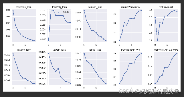
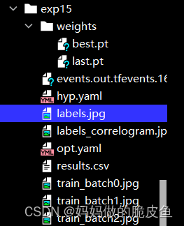
训练好的模型存放在run/train/expn目录下:
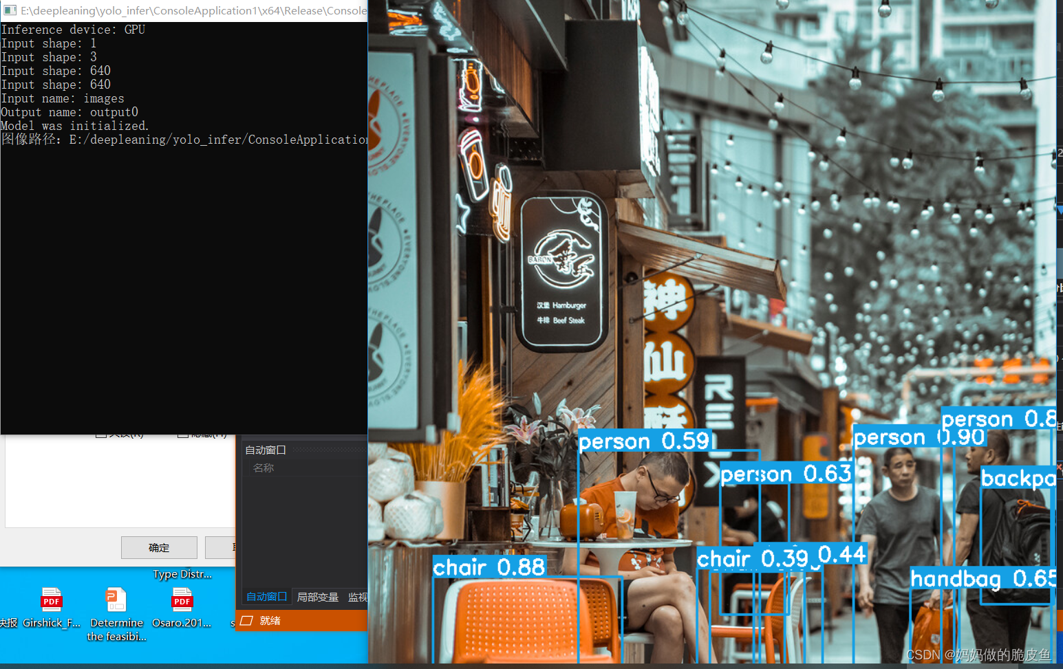
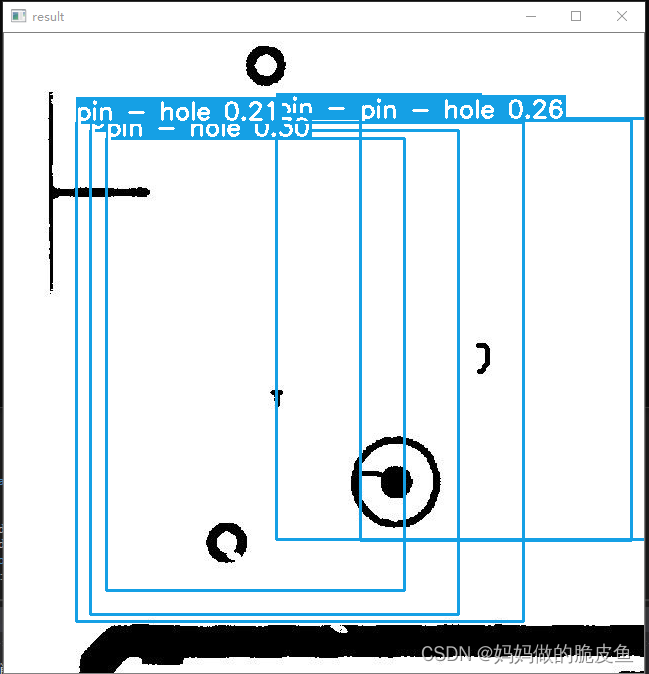
2.3.4 使用onnx runtime c++实现onnx模型的推理(部署代码可以参考onnx runtime推理yolov5)
由于只训练了10个epoch,效果不太好。(一般设置训练的epoch*nb数要大于100, 因为yolov5官方代码中, nw = max(round(hyp[‘warmup_epochs’] * nb), 100) 其中nb表示一个epoch有多少个batch,如果小于100,都还只在预热i训练阶段,效果不会很好。 )
提示:opencv提供了将图像转换为目标检测模型需要的格式的函数:
// 返回值shape: 4 - dimensional Mat with NCHW dimensions order.
cv::Mat blob = cv::dnn::blobFromImage(resizedImage, 1.0 / 255.0, resizedImage.size(), cv::Scalar(0, 0, 0), true, false, CV_32F);

// 可以使用上述函数替换void YOLODetector::preprocessing(cv::Mat &image, float*& blob, std::vector<int64_t>& inputTensorShape)函数中的图像格式转换代码。
C++模型推理代码如下所示(onnx runtime下图是基本的项目文件结构,并且以官方训练好的的yolov5模型):
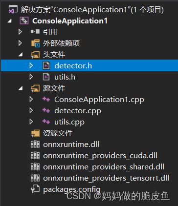
- detector.h代码
#pragma once
#include <opencv2/opencv.hpp>
#include <onnxruntime_cxx_api.h>
#include <utility>

#include "utils.h"


class YOLODetector
{


public:
	explicit YOLODetector(std::nullptr_t) {

    };
	YOLODetector(const std::string& modelPath,
		const bool& isGPU,
		const cv::Size& inputSize);

	std::vector<Detection> detect(cv::Mat &image, const float& confThreshold, const float& iouThreshold);

private:
	Ort::Env env{

     nullptr };
	Ort::SessionOptions sessionOptions{

     nullptr };
	Ort::Session session{

     nullptr };

	void preprocessing(cv::Mat &image, float*& blob, std::vector<int64_t>& inputTensorShape);
	std::vector<Detection> postprocessing(const cv::Size& resizedImageShape,
		const cv::Size& originalImageShape,
		std::vector<Ort::Value>& outputTensors,
		const float& confThreshold, const float& iouThreshold);

	static void getBestClassInfo(std::vector<float>::iterator it, const int& numClasses,
		float& bestConf, int& bestClassId);

	std::vector<const char*> inputNames;
	std::vector<const char*> outputNames;
	bool isDynamicInputShape{

    };
	cv::Size2f inputImageShape;

};
- utils.h代码
#pragma once
#include <codecvt>
#include <fstream>
#include <opencv2/opencv.hpp>


struct Detection
{


	cv::Rect box;
	float conf{

    };
	int classId{

    };
};

namespace utils
{


	size_t vectorProduct(const std::vector<int64_t>& vector);
	std::wstring charToWstring(const char* str);
	std::vector<std::string> loadNames(const std::string& path);
	void visualizeDetection(cv::Mat& image, std::vector<Detection>& detections,
		const std::vector<std::string>& classNames);

	void letterbox(const cv::Mat& image, cv::Mat& outImage,
		const cv::Size& newShape,
		const cv::Scalar& color,
		bool auto_,
		bool scaleFill,
		bool scaleUp,
		int stride);

	void scaleCoords(const cv::Size& imageShape, cv::Rect& box, const cv::Size& imageOriginalShape);

	template <typename T>
	T clip(const T& n, const T& lower, const T& upper);
}
- ConsoleApplication1.cpp代码
#include <iostream>
#include <opencv2/opencv.hpp>
#include "utils.h"
#include "detector.h"


int main(int argc, char* argv[])
{


	const float confThreshold = 0.3f;
	const float iouThreshold = 0.4f;

	YOLODetector detector{

     nullptr };
	cv::Mat image;
	std::vector<Detection> result;

	std::string modelPath = "E:/deepleaning/yolo_infer/ConsoleApplication1/ConsoleApplication1/models/yolov5s.onnx";
	bool isGPU = true;
	std::string imagePath = "E:/deepleaning/yolo_infer/ConsoleApplication1/ConsoleApplication1/images/bus.jpg";
	const std::vector<std::string> classNames = {

     "person","bicycle",
"car","motorbike","aeroplane","bus","train","truck","boat","traffic light","fire hydrant",
"stop sign","parking meter","bench","bird",
"cat","dog","horse","sheep","cow","elephant","bear","zebra","giraffe","backpack","umbrella","handbag",
"tie","suitcase","frisbee",
"skis","snowboard","sports ball","kite","baseball bat","baseball glove","skateboard","surfboard","tennis racket",
"bottle","wine glass","cup","fork","knife","spoon","bowl",
"banana",
"apple",
"sandwich",
"orange",
"broccoli",
"carrot",
"hot dog",
"pizza","donut","cake","chair","sofa","pottedplant",
"bed","diningtable","toilet","tvmonitor","laptop","mouse",
"remote","keyboard","cell phone","microwave",
"oven","toaster","sink","refrigerator",
"book","clock","vase","scissors",
"teddy bear","hair drier","toothbrush" };


	detector = YOLODetector(modelPath, isGPU, cv::Size(640, 640));
	std::cout << "Model was initialized." << std::endl;
	std::cout <<"图像路径:"<< imagePath << std::endl;

	image = cv::imread("E:/deepleaning/yolo_infer/ConsoleApplication1/ConsoleApplication1/images/bus.jpg");
	result = detector.detect(image, confThreshold, iouThreshold);
	utils::visualizeDetection(image, result, classNames);

	cv::imshow("result", image);
	cv::waitKey(0);
	return 0;
}
- detector.cpp代码
#include "detector.h"

YOLODetector::YOLODetector(const std::string& modelPath,
	const bool& isGPU = true,
	const cv::Size& inputSize = cv::Size(640, 640))
{


	env = Ort::Env(OrtLoggingLevel::ORT_LOGGING_LEVEL_WARNING, "ONNX_DETECTION");
	sessionOptions = Ort::SessionOptions();

	std::vector<std::string> availableProviders = Ort::GetAvailableProviders();
	auto cudaAvailable = std::find(availableProviders.begin(), availableProviders.end(), "CUDAExecutionProvider");
	OrtCUDAProviderOptions cudaOption;

	if (isGPU && (cudaAvailable == availableProviders.end()))
	{


		std::cout << "GPU is not supported by your ONNXRuntime build. Fallback to CPU." << std::endl;
		std::cout << "Inference device: CPU" << std::endl;
	}
	else if (isGPU && (cudaAvailable != availableProviders.end()))
	{


		std::cout << "Inference device: GPU" << std::endl;
		sessionOptions.AppendExecutionProvider_CUDA(cudaOption);
	}
	else
	{


		std::cout << "Inference device: CPU" << std::endl;
	}

#ifdef _WIN32
	std::wstring w_modelPath = utils::charToWstring(modelPath.c_str());
	session = Ort::Session(env, w_modelPath.c_str(), sessionOptions);
#else
	session = Ort::Session(env, modelPath.c_str(), sessionOptions);
#endif

	Ort::AllocatorWithDefaultOptions allocator;

	Ort::TypeInfo inputTypeInfo = session.GetInputTypeInfo(0);
	std::vector<int64_t> inputTensorShape = inputTypeInfo.GetTensorTypeAndShapeInfo().GetShape();
	this->isDynamicInputShape = false;
	// checking if width and height are dynamic
	if (inputTensorShape[2] == -1 && inputTensorShape[3] == -1)
	{


		std::cout << "Dynamic input shape" << std::endl;
		this->isDynamicInputShape = true;
	}

	for (auto shape : inputTensorShape)
		std::cout << "Input shape: " << shape << std::endl;

	inputNames.push_back(session.GetInputName(0, allocator));
	outputNames.push_back(session.GetOutputName(0, allocator));

	std::cout << "Input name: " << inputNames[0] << std::endl;
	std::cout << "Output name: " << outputNames[0] << std::endl;

	this->inputImageShape = cv::Size2f(inputSize);
}

void YOLODetector::getBestClassInfo(std::vector<float>::iterator it, const int& numClasses,
	float& bestConf, int& bestClassId)
{


	// first 5 element are box and obj confidence
	bestClassId = 5;
	bestConf = 0;

	for (int i = 5; i < numClasses + 5; i++)
	{


		if (it[i] > bestConf)
		{


			bestConf = it[i];
			bestClassId = i - 5;
		}
	}

}

void YOLODetector::preprocessing(cv::Mat &image, float*& blob, std::vector<int64_t>& inputTensorShape)
{


	cv::Mat resizedImage, floatImage;
	cv::cvtColor(image, resizedImage, cv::COLOR_BGR2RGB);
	utils::letterbox(resizedImage, resizedImage, this->inputImageShape,
		cv::Scalar(114, 114, 114), this->isDynamicInputShape,
		false, true, 32);

	inputTensorShape[2] = resizedImage.rows;
	inputTensorShape[3] = resizedImage.cols;

	resizedImage.convertTo(floatImage, CV_32FC3, 1 / 255.0);
	blob = new float[floatImage.cols * floatImage.rows * floatImage.channels()];
	cv::Size floatImageSize{

     floatImage.cols, floatImage.rows };

	// hwc -> chw
	std::vector<cv::Mat> chw(floatImage.channels());
	for (int i = 0; i < floatImage.channels(); ++i)
	{


		chw[i] = cv::Mat(floatImageSize, CV_32FC1, blob + i * floatImageSize.width * floatImageSize.height);
	}
	cv::split(floatImage, chw);
}

std::vector<Detection> YOLODetector::postprocessing(const cv::Size& resizedImageShape,
	const cv::Size& originalImageShape,
	std::vector<Ort::Value>& outputTensors,
	const float& confThreshold, const float& iouThreshold)
{


	std::vector<cv::Rect> boxes;
	std::vector<float> confs;
	std::vector<int> classIds;

	auto* rawOutput = outputTensors[0].GetTensorData<float>();
	std::vector<int64_t> outputShape = outputTensors[0].GetTensorTypeAndShapeInfo().GetShape();
	size_t count = outputTensors[0].GetTensorTypeAndShapeInfo().GetElementCount();
	std::vector<float> output(rawOutput, rawOutput + count);

	// for (const int64_t& shape : outputShape)
	//     std::cout << "Output Shape: " << shape << std::endl;

	// first 5 elements are box[4] and obj confidence
	int numClasses = (int)outputShape[2] - 5;
	int elementsInBatch = (int)(outputShape[1] * outputShape[2]);

	// only for batch size = 1
	for (auto it = output.begin(); it != output.begin() + elementsInBatch; it += outputShape[2])
	{


		float clsConf = it[4];

		if (clsConf > confThreshold)
		{


			int centerX = (int)(it[0]);
			int centerY = (int)(it[1]);
			int width = (int)(it[2]);
			int height = (int)(it[3]);
			int left = centerX - width / 2;
			int top = centerY - height / 2;

			float objConf;
			int classId;
			this->getBestClassInfo(it, numClasses, objConf, classId);

			float confidence = clsConf * objConf;

			boxes.emplace_back(left, top, width, height);
			confs.emplace_back(confidence);
			classIds.emplace_back(classId);
		}
	}

	std::vector<int> indices;
	cv::dnn::NMSBoxes(boxes, confs, confThreshold, iouThreshold, indices);
	// std::cout << "amount of NMS indices: " << indices.size() << std::endl;

	std::vector<Detection> detections;

	for (int idx : indices)
	{


		Detection det;
		det.box = cv::Rect(boxes[idx]);
		utils::scaleCoords(resizedImageShape, det.box, originalImageShape);

		det.conf = confs[idx];
		det.classId = classIds[idx];
		detections.emplace_back(det);
	}

	return detections;
}

std::vector<Detection> YOLODetector::detect(cv::Mat &image, const float& confThreshold = 0.4,
	const float& iouThreshold = 0.45)
{


	float *blob = nullptr;
	std::vector<int64_t> inputTensorShape{

     1, 3, -1, -1 };
	this->preprocessing(image, blob, inputTensorShape);

	size_t inputTensorSize = utils::vectorProduct(inputTensorShape);

	std::vector<float> inputTensorValues(blob, blob + inputTensorSize);

	std::vector<Ort::Value> inputTensors;

	Ort::MemoryInfo memoryInfo = Ort::MemoryInfo::CreateCpu(
		OrtAllocatorType::OrtArenaAllocator, OrtMemType::OrtMemTypeDefault);

	inputTensors.push_back(Ort::Value::CreateTensor<float>(
		memoryInfo, inputTensorValues.data(), inputTensorSize,
		inputTensorShape.data(), inputTensorShape.size()
		));

	std::vector<Ort::Value> outputTensors = this->session.Run(Ort::RunOptions{

     nullptr },
		inputNames.data(),
		inputTensors.data(),
		1,
		outputNames.data(),
		1);

	cv::Size resizedShape = cv::Size((int)inputTensorShape[3], (int)inputTensorShape[2]);
	std::vector<Detection> result = this->postprocessing(resizedShape,
		image.size(),
		outputTensors,
		confThreshold, iouThreshold);

	delete[] blob;

	return result;
}
- utils.cpp代码
#include "utils.h"


size_t utils::vectorProduct(const std::vector<int64_t>& vector)
{


	if (vector.empty())
		return 0;

	size_t product = 1;
	for (const auto& element : vector)
		product *= element;

	return product;
}

std::wstring utils::charToWstring(const char* str)
{


	typedef std::codecvt_utf8<wchar_t> convert_type;
	std::wstring_convert<convert_type, wchar_t> converter;

	return converter.from_bytes(str);
}

std::vector<std::string> utils::loadNames(const std::string& path)
{


	// load class names
	std::vector<std::string> classNames;
	std::ifstream infile(path);
	if (infile.good())
	{


		std::string line;
		while (getline(infile, line))
		{


			if (line.back() == '\r')
				line.pop_back();
			classNames.emplace_back(line);
		}
		infile.close();
	}
	else
	{


		std::cerr << "ERROR: Failed to access class name path: " << path << std::endl;
	}

	return classNames;
}


void utils::visualizeDetection(cv::Mat& image, std::vector<Detection>& detections,
	const std::vector<std::string>& classNames)
{


	for (const Detection& detection : detections)
	{


		cv::rectangle(image, detection.box, cv::Scalar(229, 160, 21), 2);

		int x = detection.box.x;
		int y = detection.box.y;

		int conf = (int)std::round(detection.conf * 100);
		int classId = detection.classId;
		std::string label = classNames[classId] + " 0." + std::to_string(conf);

		int baseline = 0;
		cv::Size size = cv::getTextSize(label, cv::FONT_ITALIC, 0.8, 2, &baseline);
		cv::rectangle(image,
			cv::Point(x, y - 25), cv::Point(x + size.width, y),
			cv::Scalar(229, 160, 21), -1);

		cv::putText(image, label,
			cv::Point(x, y - 3), cv::FONT_ITALIC,
			0.8, cv::Scalar(255, 255, 255), 2);
	}
}

void utils::letterbox(const cv::Mat& image, cv::Mat& outImage,
	const cv::Size& newShape = cv::Size(640, 640),
	const cv::Scalar& color = cv::Scalar(114, 114, 114),
	bool auto_ = true,
	bool scaleFill = false,
	bool scaleUp = true,
	int stride = 32)
{


	cv::Size shape = image.size();
	float r = std::min((float)newShape.height / (float)shape.height,
		(float)newShape.width / (float)shape.width);
	if (!scaleUp)
		r = std::min(r, 1.0f);

	float ratio[2]{

     r, r };
	int newUnpad[2]{

     (int)std::round((float)shape.width * r),
					 (int)std::round((float)shape.height * r) };

	auto dw = (float)(newShape.width - newUnpad[0]);
	auto dh = (float)(newShape.height - newUnpad[1]);

	if (auto_)
	{


		dw = (float)((int)dw % stride);
		dh = (float)((int)dh % stride);
	}
	else if (scaleFill)
	{


		dw = 0.0f;
		dh = 0.0f;
		newUnpad[0] = newShape.width;
		newUnpad[1] = newShape.height;
		ratio[0] = (float)newShape.width / (float)shape.width;
		ratio[1] = (float)newShape.height / (float)shape.height;
	}

	dw /= 2.0f;
	dh /= 2.0f;

	if (shape.width != newUnpad[0] && shape.height != newUnpad[1])
	{


		cv::resize(image, outImage, cv::Size(newUnpad[0], newUnpad[1]));
	}

	int top = int(std::round(dh - 0.1f));
	int bottom = int(std::round(dh + 0.1f));
	int left = int(std::round(dw - 0.1f));
	int right = int(std::round(dw + 0.1f));
	cv::copyMakeBorder(outImage, outImage, top, bottom, left, right, cv::BORDER_CONSTANT, color);
}

void utils::scaleCoords(const cv::Size& imageShape, cv::Rect& coords, const cv::Size& imageOriginalShape)
{


	float gain = std::min((float)imageShape.height / (float)imageOriginalShape.height,
		(float)imageShape.width / (float)imageOriginalShape.width);

	int pad[2] = {

     (int)(((float)imageShape.width - (float)imageOriginalShape.width * gain) / 2.0f),
				  (int)(((float)imageShape.height - (float)imageOriginalShape.height * gain) / 2.0f) };

	coords.x = (int)std::round(((float)(coords.x - pad[0]) / gain));
	coords.y = (int)std::round(((float)(coords.y - pad[1]) / gain));

	coords.width = (int)std::round(((float)coords.width / gain));
	coords.height = (int)std::round(((float)coords.height / gain));

}
template <typename T>
T utils::clip(const T& n, const T& lower, const T& upper)
{


	return std::max(lower, std::min(n, upper));
}