深度学习论文: A Zero-/Few-Shot Anomaly Classification and Segmentation Method for CVPR 2023 VAND Workshop

深度学习论文: A Zero-/Few-Shot Anomaly Classification and Segmentation Method for CVPR 2023 VAND Workshop Challenge Tracks 1&2: 1st Place on Zero-shot AD and 4th Place on Few-shot AD
A Zero-/Few-Shot Anomaly Classification and Segmentation Method for CVPR 2023 VAND Workshop Challenge Tracks 1&2: 1st Place on Zero-shot AD and 4th Place on Few-shot AD
PDF: https://arxiv.org/pdf/2305.17382.pdf
PyTorch代码: https://github.com/shanglianlm0525/CvPytorch
PyTorch代码: https://github.com/shanglianlm0525/PyTorch-Networks

1 概述

为了解决工业视觉检测中产品类型的广泛多样性，我们构建一个可以快速适应众多类别且不需要或只需要很少的正常参考图像的单一模型，为工业视觉检测提供更加高效的解决方案。提出了针对2023年VAND挑战的零/少样本跟踪的解决方案。

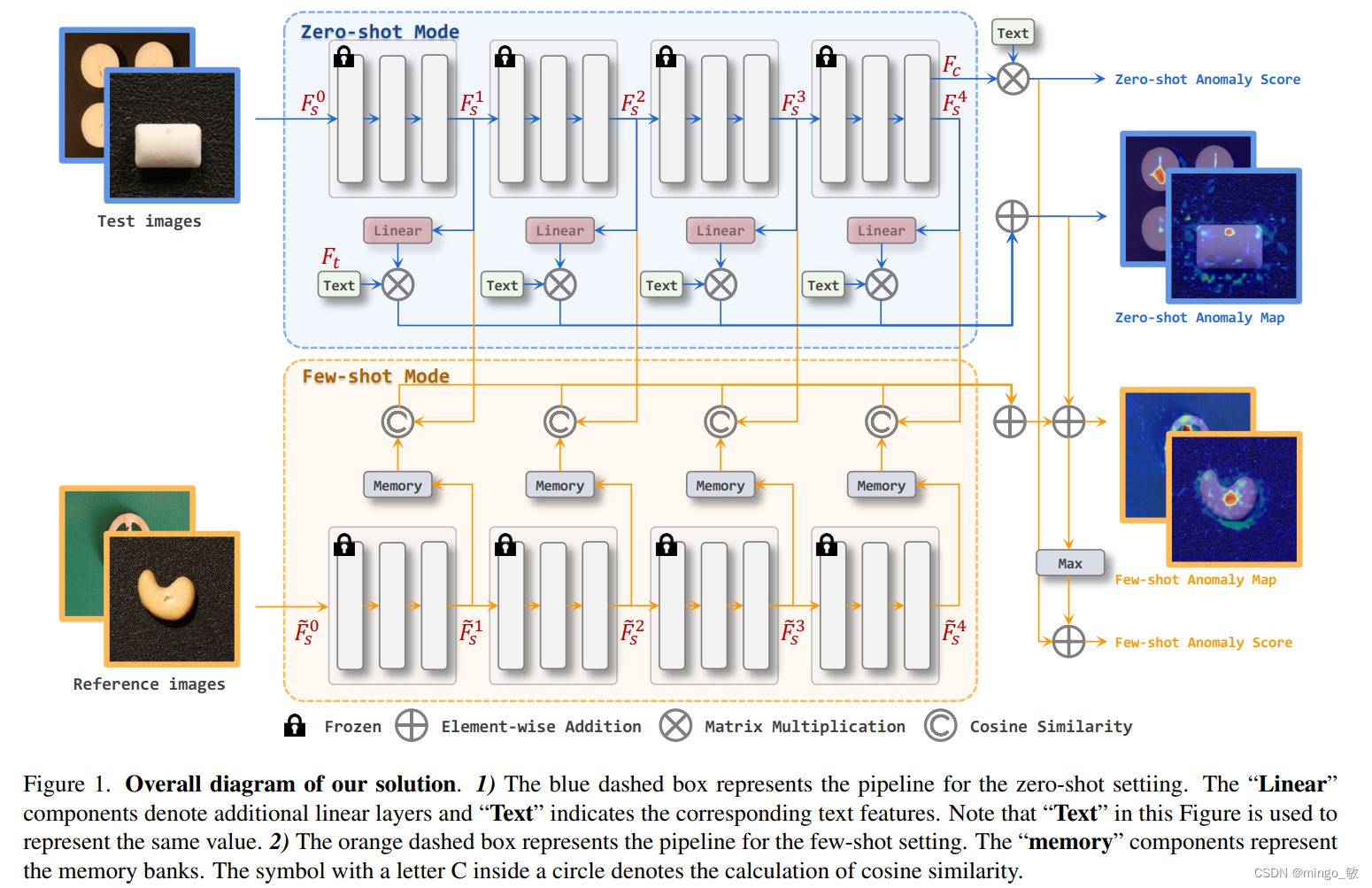
1）在zero-shot任务中，所提解决方案在CLIP模型上加入额外的线形层，使图像特征映射到联合嵌入空间，从而使其能够与文本特征进行比较并生成异anomaly maps。
2）当有参考图像可用时（few-shot），所提解决方案利用多个memory banks存储参考图像特征，并在测试时与查询图像进行比较。

在这个挑战中，我们的方法在Zero-Shot中取得了第一名，并在分割方面表现出色，F1得分比第二名参赛者提高了0.0489。在Few-Shot中，我们在总体排名中获得了第四名，在分类F1得分方面排名第一。

核心要点：

使用状态（state）和模板（template）的提示集成来制作文本提示。
为了定位异常区域，引入了额外的线性层，将从CLIP图像编码器提取的图像特征映射到文本特征所在的线性空间。
将映射的图像特征与文本特征进行相似度比较，从而得到相应的anomaly maps。
few-shot中，保留zero-shot阶段的额外线性层并保持它们的权重。此外，在测试阶段使用图像编码器提取参考图像的特征并保存到memory banks中，以便与测试图像的特征进行比较。
为了充分利用浅层和深层特征，同时利用了图像编码器不同stage的特征。

2 Methodology

总的来说，我们采用了CLIP的整体框架进行零样本分类，并使用状态和模板集合的组合来构建我们的文本提示。为了定位图像中的异常区域，我们引入了额外的线性层，将从CLIP图像编码器中提取的图像特征映射到文本特征所在的线性空间中。然后，我们对映射后的图像特征和文本特征进行相似性比较，以获取相应的异常图。对于少样本情况，我们保留零样本阶段的额外线性层并保持它们的权重。此外，我们使用图像编码器提取参考图像的特征并将其保存到内存库中，在测试阶段将其与测试图像的特征进行比较。需要注意的是，为了充分利用浅层和深层特征，我们在零本和少样本设置中都使用来自不同阶段的特征。

在这里插入图片描述

2-1 Zero-shot AD

Anomaly Classification
基于WinCLIP 异常分类框架，我们提出了一种文本提示集成策略，在不使用复杂的多尺度窗口策略的基础上显著提升了Baseline的异常分类精度。具体地，该集成策略包含template-level和state-level两部分：
1）state-level文本提示是使用通用的文本描述正常或异常的目标（比如flawless,damaged），而不会使用“chip around edge and corner”这种过于细节的描述；
2）template-level文本提示，所提方案在CLIP中为ImageNet筛选了85个模板，并移除了“a photo of the weird [obj.]”等不适用于异常检测任务的模板。
这两种文本提示将通过CLIP的文本编码器提取为最终的文本特征： $F_{t} \in R^{2 \times C}$ 。

def encode_text_with_prompt_ensemble(model, texts, device):
    prompt_normal = ['{}', 'flawless {}', 'perfect {}', 'unblemished {}', '{} without flaw', '{} without defect', '{} without damage']
    prompt_abnormal = ['damaged {}', 'broken {}', '{} with flaw', '{} with defect', '{} with damage']
    prompt_state = [prompt_normal, prompt_abnormal]
    prompt_templates = ['a bad photo of a {}.', 
                        'a low resolution photo of the {}.', 
                        'a bad photo of the {}.', 
                        'a cropped photo of the {}.', 
                        'a bright photo of a {}.', 
                        'a dark photo of the {}.', 
                        'a photo of my {}.', 
                        'a photo of the cool {}.', 
                        'a close-up photo of a {}.', 
                        'a black and white photo of the {}.', 
                        'a bright photo of the {}.', 
                        'a cropped photo of a {}.', 
                        'a jpeg corrupted photo of a {}.', 
                        'a blurry photo of the {}.', 
                        'a photo of the {}.', 
                        'a good photo of the {}.', 
                        'a photo of one {}.', 
                        'a close-up photo of the {}.', 
                        'a photo of a {}.', 
                        'a low resolution photo of a {}.', 
                        'a photo of a large {}.', 
                        'a blurry photo of a {}.', 
                        'a jpeg corrupted photo of the {}.', 
                        'a good photo of a {}.', 
                        'a photo of the small {}.', 
                        'a photo of the large {}.', 
                        'a black and white photo of a {}.', 
                        'a dark photo of a {}.', 
                        'a photo of a cool {}.', 
                        'a photo of a small {}.', 
                        'there is a {} in the scene.', 
                        'there is the {} in the scene.', 
                        'this is a {} in the scene.', 
                        'this is the {} in the scene.', 
                        'this is one {} in the scene.']

    text_features = []
    for i in range(len(prompt_state)):
        prompted_state = [state.format(texts[0]) for state in prompt_state[i]]
        prompted_sentence = []
        for s in prompted_state: # [prompt_normal, prompt_abnormal]
            for template in prompt_templates:
                prompted_sentence.append(template.format(s))
        prompted_sentence = tokenize(prompted_sentence).to(device)
        class_embeddings = model.encode_text(prompted_sentence)
        class_embeddings /= class_embeddings.norm(dim=-1, keepdim=True)
        class_embedding = class_embeddings.mean(dim=0)
        class_embedding /= class_embedding.norm()
        text_features.append(class_embedding)
    text_features = torch.stack(text_features, dim=1).to(device).t()

    return text_features

对应的图像特征经图像编码器为： $F_{c} \in R^{1 \times C}$ 。
state-level和template-level的集成实现, 使用CLIP文本编码器提取文本特征，并对正常和异常特征分别求平均值。最终，将正常与异常特征各自的平均值与图像特征进行对比，经过softmax后得到异常类别概率作为分类得分
$s = softmax(F_{c}F_{t}^{T})$
最后选择 $s$ 的第二维度作为异常检测分类问题的结果。

text_probs = (100.0 * image_features @ text_features.T).softmax(dim=-1)
results['pr_sp'].append(text_probs[0][1].cpu().item())

Anomaly Segmentation
类比图像级别的异常分类方法到异常分割，一个自然而然的想法是将Backbone提取到的不同层级特征与文本特征进行相似度度量。然而，CLIP模型是基于分类的方案进行设计的，即除了用于分类的抽象图像特征外，没有将其它图像特征映射到统一的图像/文本空间。因此我们提出了一个简单但有效的方案来解决这个问题：使用额外的线性层将不同层级的图像特征映射到图像/文本联合嵌入空间中，即linear layer去映射patch_tokens，然后基于每个patch_token去和文本特征做相似度计算，从而得到anomaly map。，见上图中蓝色Zero-shot Anomaly Map流程。具体地，不同层级的特征分别经由一个线性层进行联合嵌入特征空间变换，将得到的变换后的特征与文本特征进行对比，得到不同层级的异常图。最后，将不同层级的异常图简单加和求得最终结果。

patch_tokens = linearlayer(patch_tokens)
anomaly_maps = []
for layer in range(len(patch_tokens)):
  patch_tokens[layer] /= patch_tokens[layer].norm(dim=-1, keepdim=True)
  anomaly_map = (100.0 * patch_tokens[layer] @ text_features.T)
  B, L, C = anomaly_map.shape
  H = int(np.sqrt(L))
  anomaly_map = F.interpolate(anomaly_map.permute(0, 2, 1).view(B, 2, H, H),
  size=img_size, mode='bilinear', align_corners=True)
  anomaly_map = torch.softmax(anomaly_map, dim=1)[:, 1, :, :]
  anomaly_maps.append(anomaly_map.cpu().numpy())
anomaly_map = np.sum(anomaly_maps, axis=0)

Linear Layer的训练（CLIP部分的参数是冻结的）使用了focal loss和dice loss。

2-2 Few-shot AD

Anomaly Classification
对于few-shot设置，图像的异常预测来自两部分。第一部分与zero-shot设置相同。第二部分遵循许多AD方法中使用的常规方法，考虑anomaly map的最大值。所提方案将这两部分相加作为最终的异常得分。

Anomaly Segmentation
few-shot分割任务使用了memory bank，如图1中的黄色背景部分。
直白来说，就是查询样本和memory bank中的支持样本去做余弦相似度，再通过reshape得到anomaly map，最后再加到zero-shot得到的anomaly map上得到最后的分割预测。
另外在few-shot任务中没有再去fine-tune上文提到的linear layer，而是直接使用了zero-shot任务中训练好的权重。

3 Experiments

在这里插入图片描述
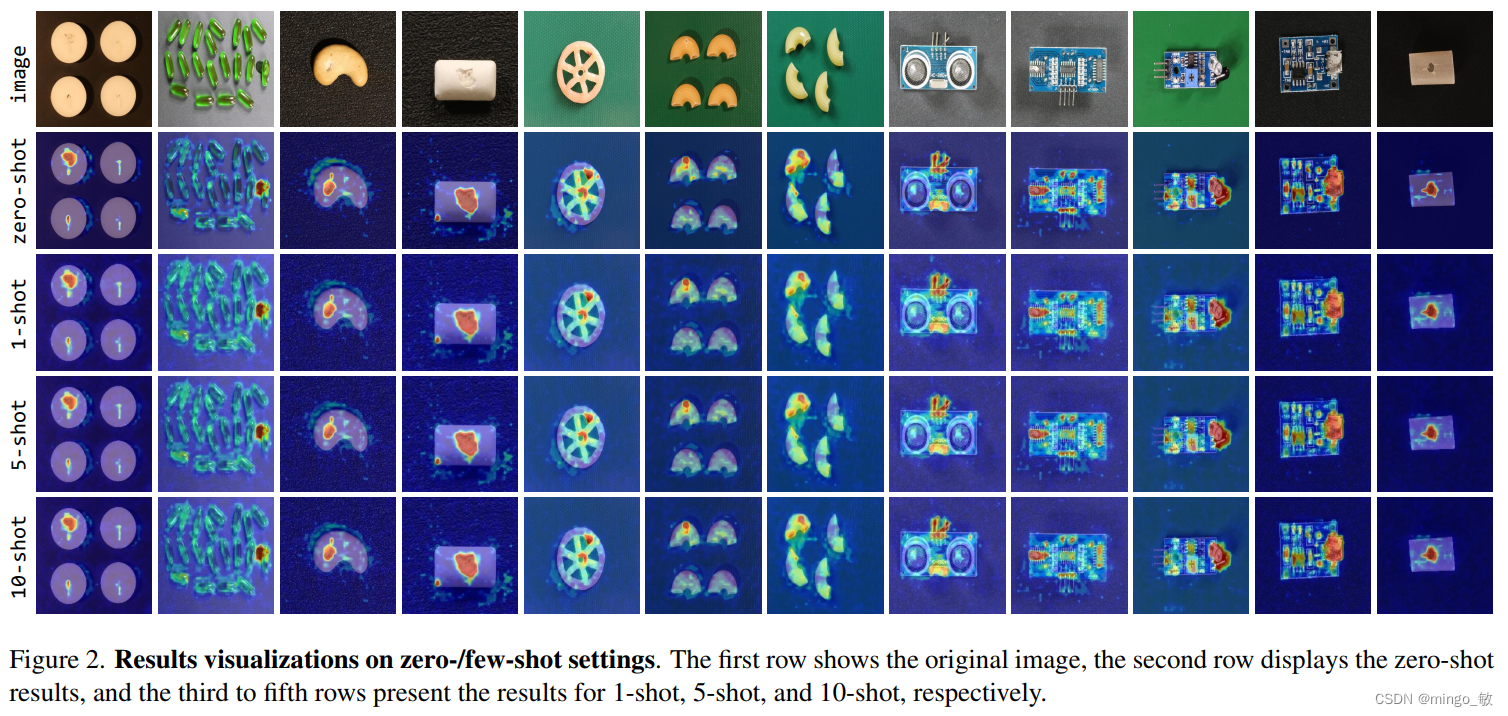
简单来说，在简单一些的图像中zero-shot和few-shot上效果差不多，但面对困难任务时，few-shot会改善一些。