PL-VINS线特征处理部分源码阅读

本文主要阅读PL-VINS中引入线特征的代码实现，包括线特征表示方法（Plücker参数化方法、正交表示法）、前端线特征提取与匹配、三角化、后端优化等。

公式推导参考：SLAM中线特征的参数化和求导

1 linefeature_tracker

linefeature_tracker_node的整体结构跟feature_tracker_node基本一致，主要处理在readImage，用LSD作线特征提取，LBD做描述子匹配，这部分处理都是直接调用opencv接口实现的。

LSD线特征提取
设置了一些提取参数和阈值，特别是针对线段长度做了筛选。

Ptr<line_descriptor::LSDDetectorC> lsd_ = line_descriptor::LSDDetectorC::createLSDDetectorC();
    // lsd parameters
    line_descriptor::LSDDetectorC::LSDOptions opts;
    opts.refine       = 1;     //1     	The way found lines will be refined
    opts.scale        = 0.5;   //0.8   	The scale of the image that will be used to find the lines. Range (0..1].
    opts.sigma_scale  = 0.6;	//0.6  	Sigma for Gaussian filter. It is computed as sigma = _sigma_scale/_scale.
    opts.quant        = 2.0;	//2.0   Bound to the quantization error on the gradient norm
    opts.ang_th       = 22.5;	//22.5	Gradient angle tolerance in degrees
    opts.log_eps      = 1.0;	//0		Detection threshold: -log10(NFA) > log_eps. Used only when advance refinement is chosen
    opts.density_th   = 0.6;	//0.7	Minimal density of aligned region points in the enclosing rectangle.
    opts.n_bins       = 1024;	//1024 	Number of bins in pseudo-ordering of gradient modulus.
    double min_line_length = 0.125;  // Line segments shorter than that are rejected
    // opts.refine       = 1;
    // opts.scale        = 0.5;
    // opts.sigma_scale  = 0.6;
    // opts.quant        = 2.0;
    // opts.ang_th       = 22.5;
    // opts.log_eps      = 1.0;
    // opts.density_th   = 0.6;
    // opts.n_bins       = 1024;
    // double min_line_length = 0.125;
    opts.min_length   = min_line_length*(std::min(img.cols,img.rows));

    std::vector<KeyLine> lsd, keylsd;
	//void LSDDetectorC::detect( const std::vector<Mat>& images, std::vector<std::vector<KeyLine> >& keylines, int scale, int numOctaves, const std::vector<Mat>& masks ) const
    lsd_->detect( img, lsd, 2, 1, opts);

LBD描述子匹配筛选

做了一个匹配筛选，认为连续两帧中，同一个线段不会发生很大的移动，所以直接比较了两个端点的像素坐标和两个线段的夹角。

Point2f serr = line1.getStartPoint() - line2.getEndPoint()这一句可能是写错了，猜测是line2.getStartPoint()

if(curframe_->keylsd.size() > 0)
    {
    
    
        /* compute matches */
        TicToc t_match;
        std::vector<DMatch> lsd_matches;
        Ptr<BinaryDescriptorMatcher> bdm_;
        bdm_ = BinaryDescriptorMatcher::createBinaryDescriptorMatcher();
        bdm_->match(forwframe_->lbd_descr, curframe_->lbd_descr, lsd_matches);
//        ROS_INFO("lbd_macht costs: %fms", t_match.toc());
        sum_time += t_match.toc();
        mean_time = sum_time/frame_cnt;
        // ROS_INFO("line feature tracker mean costs: %fms", mean_time);
        /* select best matches */
        std::vector<DMatch> good_matches;
        std::vector<KeyLine> good_Keylines;
        good_matches.clear();
        for ( int i = 0; i < (int) lsd_matches.size(); i++ )
        {
    
    
            if( lsd_matches[i].distance < 30 ){
    
    

                DMatch mt = lsd_matches[i];
                KeyLine line1 =  forwframe_->keylsd[mt.queryIdx] ;
                KeyLine line2 =  curframe_->keylsd[mt.trainIdx] ;
                Point2f serr = line1.getStartPoint() - line2.getEndPoint();
                Point2f eerr = line1.getEndPoint() - line2.getEndPoint();
                // std::cout<<"11111111111111111 = "<<abs(line1.angle-line2.angle)<<std::endl;
                if((serr.dot(serr) < 200 * 200) && (eerr.dot(eerr) < 200 * 200)&&abs(line1.angle-line2.angle)<0.1)   // 线段在图像里不会跑得特别远
                    good_matches.push_back( lsd_matches[i] );
            }
        }


        vector< int > success_id;
        // std::cout << forwframe_->lineID.size() <<" " <<curframe_->lineID.size();
        for (int k = 0; k < good_matches.size(); ++k) {
    
    
            DMatch mt = good_matches[k];
            forwframe_->lineID[mt.queryIdx] = curframe_->lineID[mt.trainIdx];
            success_id.push_back(curframe_->lineID[mt.trainIdx]);
        }

坐标归一化

trackerData.undistortedLineEndPoints()操作后，得到当前帧下所有线特征起点和终点的归一化坐标（我感觉这个函数本意应该是要做去畸变的，结果代码里只做了像素坐标转归一化坐标，这样一来线特征不就没有去畸变吗？）

然后把id和归一化坐标pub出去

    pub_img = n.advertise<sensor_msgs::PointCloud>("linefeature", 1000);
    pub_match = n.advertise<sensor_msgs::Image>("linefeature_img",1000);

这版里面pub_match完全没用到啊，类比feature_tracker，猜测是留给双目显示左右目匹配用的。

2 三角化

三角化放在了里程计处理部分，一共有三种方案：

• 点特征三角化（SFM）
• 单目线特征三角化（SFM）
• 双目线特征三角化

void Estimator::solveOdometry()
{
    
    
    if (frame_count < WINDOW_SIZE)
        return;
    if (solver_flag == NON_LINEAR)
    {
    
    
        TicToc t_tri;
        f_manager.triangulate(Ps, tic, ric);

        if(baseline_ > 0) //stereo
            f_manager.triangulateLine(baseline_);
        else
            f_manager.triangulateLine(Ps, tic, ric);

        ROS_DEBUG("triangulation costs %f", t_tri.toc());

        // optimization();

        onlyLineOpt();   // 三角化以后，优化一把
        optimizationwithLine();

#ifdef LINEINCAM
        LineBAincamera();
#else
//        LineBA();
#endif
    }
}

单目三角化

单目情况下线特征三角化同样是通过SFM实现。
通过ij两帧图像观测到的线段头尾端点，与当前帧相机坐标原点的连线，构造观测平面，两平面相交得到相机坐标系下的直线Lc。

分为下图两种情况：

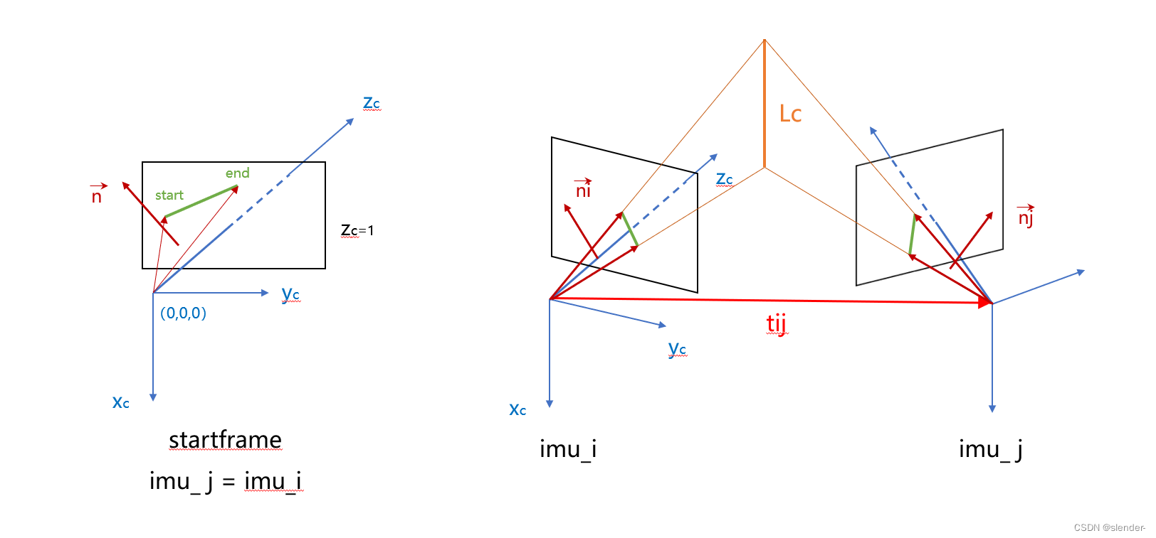
情况1：imu_j == imu_i 直接计算跟光心连线构成的平面法向量

           if(imu_j == imu_i)   // 第一个观测是start frame 上
            {
    
    
                obsi = it_per_frame.lineobs;
                Eigen::Vector3d p1( obsi(0), obsi(1), 1 );
                Eigen::Vector3d p2( obsi(2), obsi(3), 1 );
                pii = pi_from_ppp(p1, p2,Vector3d( 0, 0, 0 ));
                ni = pii.head(3); ni.normalize();
                continue;
            }

情况2：imu_j ！= imu_i 算出第i帧图像坐标系下，第j帧图像的线段与光心构成的平面法向量

// 非start frame(其他帧)上的观测
            Eigen::Vector3d t1 = Ps[imu_j] + Rs[imu_j] * tic[0];
            Eigen::Matrix3d R1 = Rs[imu_j] * ric[0];

            Eigen::Vector3d t = R0.transpose() * (t1 - t0);   // tij
            Eigen::Matrix3d R = R0.transpose() * R1;          // Rij
            
            Eigen::Vector4d obsj_tmp = it_per_frame.lineobs;

            // plane pi from jth obs in ith camera frame
            Vector3d p3( obsj_tmp(0), obsj_tmp(1), 1 );
            Vector3d p4( obsj_tmp(2), obsj_tmp(3), 1 );
            p3 = R * p3 + t;
            p4 = R * p4 + t;
            Vector4d pij = pi_from_ppp(p3, p4,t);
            Eigen::Vector3d nj = pij.head(3); nj.normalize(); 

两平面相交，得到相机坐标系下直线的普朗克表示

Vector6d plk = pipi_plk( pii, pij );
Vector3d n = plk.head(3);
Vector3d v = plk.tail(3);
it_per_id.line_plucker = plk;  // plk in camera frame
it_per_id.is_triangulation = true;

双目三角化

双目更简单，把线段与左右目构成的平面相交。

来自论文《Building a 3-D Line-Based Map Using Stereo SLAM》

   // plane pi from ith left obs in ith left camera frame
        Vector3d p1( lineobs_l(0), lineobs_l(1), 1 );
        Vector3d p2( lineobs_l(2), lineobs_l(3), 1 );
        Vector4d pii = pi_from_ppp(p1, p2,Vector3d( 0, 0, 0 ));

        // plane pi from ith right obs in ith left camera frame
        Vector3d p3( lineobs_r(0) + baseline, lineobs_r(1), 1 );
        Vector3d p4( lineobs_r(2) + baseline, lineobs_r(3), 1 );
        Vector4d pij = pi_from_ppp(p3, p4,Vector3d(baseline, 0, 0));

        Vector6d plk = pipi_plk( pii, pij );
        Vector3d n = plk.head(3);
        Vector3d v = plk.tail(3);

3 后端优化

做完三角化之后，先做了一次线特征的优化onlyLineOpt()，然后做了滑窗整体的优化optimizationwithLine()

• onlyLineOpt() 固定pose， 只优化line
• optimizationwithLine() 优化pose、imu、feature(points and lines)

线特征状态量

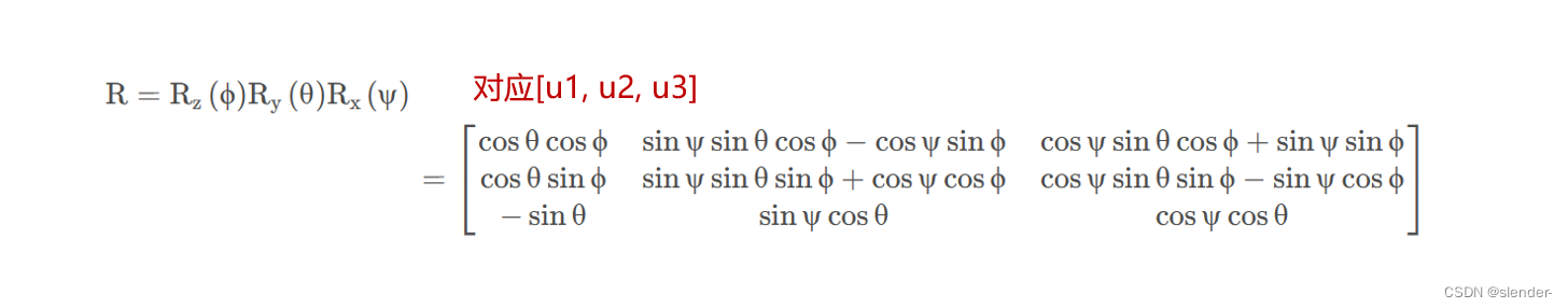
在优化部分，作者把线特征从普朗克表示（6x1）转为正交表示（4x1），在plk_to_orth 实现.
这样做主要是因为直线的自由度是4，而普朗克表示是冗余的。

引用自论文《PLS-VIO_Stereo_Vision-inertial_Odometry_Based_on_Point_and_Line_Features》

Vector4d plk_to_orth(Vector6d plk)
{
    
    
    Vector4d orth;
    Vector3d n = plk.head(3);
    Vector3d v = plk.tail(3);

    Vector3d u1 = n/n.norm();
    Vector3d u2 = v/v.norm();
    Vector3d u3 = u1.cross(u2);

    // todo:: use SO3
    orth[0] = atan2( u2(2),u3(2) );
    orth[1] = asin( -u1(2) );
    orth[2] = atan2( u1(1),u1(0) );

    Vector2d w( n.norm(), v.norm() );
    w = w/w.norm();
    orth[3] = asin( w(1) );

    return orth;

}

重投影误差

这里的重投影误差是把世界坐标系下的直线投影到归一化平面上，然后计算之前提取的线段两端点坐标到直线投影的距离，理想情况下是0。

注意，重投影误差是在归一化平面进行的，与相机内参无关。

ceres::LocalParameterization *local_parameterization_line = new LineOrthParameterization();
        problem.AddParameterBlock( para_LineFeature[linefeature_index], SIZE_LINE, local_parameterization_line);  // p,q

        int imu_i = it_per_id.start_frame,imu_j = imu_i - 1;
        for (auto &it_per_frame : it_per_id.linefeature_per_frame)
        {
    
    
            imu_j++;
            if (imu_i == imu_j)
            {
    
    
                //continue;
            }
            Vector4d obs = it_per_frame.lineobs;                          // 在第j帧图像上的观测
            lineProjectionFactor *f = new lineProjectionFactor(obs);     // 特征重投影误差
            problem.AddResidualBlock(f, loss_function,
                                     para_Pose[imu_j],
                                     para_Ex_Pose[0],
                                     para_LineFeature[linefeature_index]);
            line_m_cnt++;
        }

重投影误差计算过程：

1. 正交表示法→普朗克表示法
2. 世界坐标系→b系→相机系→相机归一化坐标系
3. 根据点到直线距离公式计算残差项

论文《PL-VIO: Tightly-Coupled Monocular Visual–Inertial Odometry Using Point and Line Features》中提到，当直线从相机系投影到归一化坐标系下，投影参数K是单位阵。

如果是投影到像素坐标系，就采用下面这个投影矩阵。

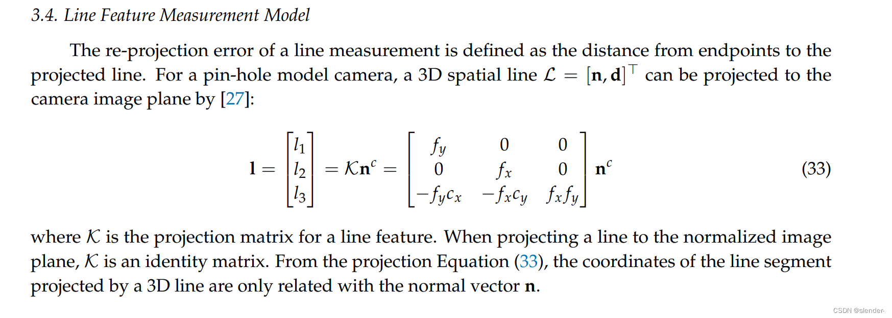
这里的[l1, l2, l3]T，就是直线参数abc，然后带入点到直线距离公式：

论文写的线段中点，代码用的起始和末尾俩端点，没啥区别。

bool lineProjectionFactor::Evaluate(double const *const *parameters, double *residuals, double **jacobians) const
{
    
    
    Eigen::Vector3d Pi(parameters[0][0], parameters[0][1], parameters[0][2]);
    Eigen::Quaterniond Qi(parameters[0][6], parameters[0][3], parameters[0][4], parameters[0][5]);

    Eigen::Vector3d tic(parameters[1][0], parameters[1][1], parameters[1][2]);
    Eigen::Quaterniond qic(parameters[1][6], parameters[1][3], parameters[1][4], parameters[1][5]);

    Eigen::Vector4d line_orth( parameters[2][0],parameters[2][1],parameters[2][2],parameters[2][3]);
    Vector6d line_w = orth_to_plk(line_orth);

    Eigen::Matrix3d Rwb(Qi);
    Eigen::Vector3d twb(Pi);
    Vector6d line_b = plk_from_pose(line_w, Rwb, twb);
    //std::cout << line_b.norm() <<"\n";
    Eigen::Matrix3d Rbc(qic);
    Eigen::Vector3d tbc(tic);
    Vector6d line_c = plk_from_pose(line_b, Rbc, tbc);

    // 直线的投影矩阵K为单位阵
    Eigen::Vector3d nc = line_c.head(3);
    double l_norm = nc(0) * nc(0) + nc(1) * nc(1);
    double l_sqrtnorm = sqrt( l_norm );
    double l_trinorm = l_norm * l_sqrtnorm;

    double e1 = obs_i(0) * nc(0) + obs_i(1) * nc(1) + nc(2);
    double e2 = obs_i(2) * nc(0) + obs_i(3) * nc(1) + nc(2);
    Eigen::Map<Eigen::Vector2d> residual(residuals);
    residual(0) = e1/l_sqrtnorm;
    residual(1) = e2/l_sqrtnorm;

//    std::cout <<"---- sqrt_info: ------"<< sqrt_info << std::endl;
//    sqrt_info.setIdentity();
    residual = sqrt_info * residual;
    //std::cout << residual <<"\n";
    if (jacobians)
    {
    
    

        Eigen::Matrix<double, 2, 3> jaco_e_l(2, 3);
        jaco_e_l << (obs_i(0)/l_sqrtnorm - nc(0) * e1 / l_trinorm ), (obs_i(1)/l_sqrtnorm - nc(1) * e1 / l_trinorm ), 1.0/l_sqrtnorm,
                (obs_i(2)/l_sqrtnorm - nc(0) * e2 / l_trinorm ), (obs_i(3)/l_sqrtnorm - nc(1) * e2 / l_trinorm ), 1.0/l_sqrtnorm;

        jaco_e_l = sqrt_info * jaco_e_l;

        Eigen::Matrix<double, 3, 6> jaco_l_Lc(3, 6);
        jaco_l_Lc.setZero();
        jaco_l_Lc.block(0,0,3,3) = Eigen::Matrix3d::Identity();

        Eigen::Matrix<double, 2, 6> jaco_e_Lc;
        jaco_e_Lc = jaco_e_l * jaco_l_Lc;
        //std::cout <<jaco_e_Lc<<"\n\n";
        //std::cout << "jacobian_calculator:" << std::endl;
        if (jacobians[0])
        {
    
    
            //std::cout <<"jacobian_pose_i"<<"\n";
            Eigen::Map<Eigen::Matrix<double, 2, 7, Eigen::RowMajor>> jacobian_pose_i(jacobians[0]);

            Matrix6d invTbc;
            invTbc << Rbc.transpose(), -Rbc.transpose()*skew_symmetric(tbc),
                    Eigen::Matrix3d::Zero(),  Rbc.transpose();

            Vector3d nw = line_w.head(3);
            Vector3d dw = line_w.tail(3);
            Eigen::Matrix<double, 6, 6> jaco_Lc_pose;
            jaco_Lc_pose.setZero();
            jaco_Lc_pose.block(0,0,3,3) = Rwb.transpose() * skew_symmetric(dw);   // Lc_t
            jaco_Lc_pose.block(0,3,3,3) = skew_symmetric( Rwb.transpose() * (nw + skew_symmetric(dw) * twb) );  // Lc_theta
            jaco_Lc_pose.block(3,3,3,3) = skew_symmetric( Rwb.transpose() * dw);

            jaco_Lc_pose = invTbc * jaco_Lc_pose;
            //std::cout <<invTbc<<"\n"<<jaco_Lc_pose<<"\n\n";

            jacobian_pose_i.leftCols<6>() = jaco_e_Lc * jaco_Lc_pose;

            //std::cout <<jacobian_pose_i<<"\n\n";

            jacobian_pose_i.rightCols<1>().setZero();            //最后一列设成0
        }

        if (jacobians[1])
        {
    
    

            //std::cout <<"jacobian_ex_pose"<<"\n";
            Eigen::Map<Eigen::Matrix<double, 2, 7, Eigen::RowMajor>> jacobian_ex_pose(jacobians[1]);

            Vector3d nb = line_b.head(3);
            Vector3d db = line_b.tail(3);
            Eigen::Matrix<double, 6, 6> jaco_Lc_ex;
            jaco_Lc_ex.setZero();
            jaco_Lc_ex.block(0,0,3,3) = Rbc.transpose() * skew_symmetric(db);   // Lc_t
            jaco_Lc_ex.block(0,3,3,3) = skew_symmetric( Rbc.transpose() * (nb + skew_symmetric(db) * tbc) );  // Lc_theta
            jaco_Lc_ex.block(3,3,3,3) = skew_symmetric( Rbc.transpose() * db);

            jacobian_ex_pose.leftCols<6>() = jaco_e_Lc * jaco_Lc_ex;
            jacobian_ex_pose.rightCols<1>().setZero();
        }
        if (jacobians[2])
        {
    
    
            Eigen::Map<Eigen::Matrix<double, 2, 4, Eigen::RowMajor>> jacobian_lineOrth(jacobians[2]);

            Eigen::Matrix3d Rwc = Rwb * Rbc;
            Eigen::Vector3d twc = Rwb * tbc + twb;
            Matrix6d invTwc;
            invTwc << Rwc.transpose(), -Rwc.transpose() * skew_symmetric(twc),
                    Eigen::Matrix3d::Zero(),  Rwc.transpose();
            //std::cout<<invTwc<<"\n";

            Vector3d nw = line_w.head(3);
            Vector3d vw = line_w.tail(3);
            Vector3d u1 = nw/nw.norm();
            Vector3d u2 = vw/vw.norm();
            Vector3d u3 = u1.cross(u2);
            Vector2d w( nw.norm(), vw.norm() );
            w = w/w.norm();

            Eigen::Matrix<double, 6, 4> jaco_Lw_orth;
            jaco_Lw_orth.setZero();
            jaco_Lw_orth.block(3,0,3,1) = w[1] * u3;
            jaco_Lw_orth.block(0,1,3,1) = -w[0] * u3;
            jaco_Lw_orth.block(0,2,3,1) = w(0) * u2;
            jaco_Lw_orth.block(3,2,3,1) = -w(1) * u1;
            jaco_Lw_orth.block(0,3,3,1) = -w(1) * u1;
            jaco_Lw_orth.block(3,3,3,1) = w(0) * u2;

            //std::cout<<jaco_Lw_orth<<"\n";

            jacobian_lineOrth = jaco_e_Lc * invTwc * jaco_Lw_orth;
        }

    }

这里还有一个要留意的点，在计算点到直线距离的时候，直线abc参数直接就是法向量参数。

光心与相机坐标系下的线特征两端连线，构成一个平面并且得到这个平面的法向量。那为什么这个法向量就是归一化平面上投影直线的参数呢？

法向量n=[n1, n2, n3]，对于投影直线上的一个点(x, y, z)， 这个点位于归一化平面上z=1，同时位于法向量所在平面上，所以就有 n1x+n2y+n3=0，对应了直线表达式 ax+by+c=0。

这也解释了为什么投影矩阵为单位阵，它的投影过程只与法向量有关，在这个过程中法向量并不发生变化。