HALCON：Optical Flow（光流法）

光流法基本原理

光流概念由Gibson在1950年首先提出来，它是一种简单实用的图像运动表达方式，通常定义为一个图像序列中图像亮度模式的表观运动，即空间物体表面上点的运动速度在视觉传感器成像平面上的表达，是利用图像序列中像素在时间域上的变化以及相邻帧之间的相关性来找到上一帧跟当前帧之间存在的对应关系，从而计算出相邻帧之间物体的运动信息的一种方法。这种定义认为光流只表示一种几何变化。1998年Negahdaripour将光流重新定义为动态图像几何变化和辐射度变化的全面表示。光流研究是利用图像序列中像素强度数据的时域变化和相关性来确定各自像素位置的“运动”，即研究图像灰度在时间上的变化与景象中物体结构及其运动的关系。一般情况下，光流由相机运动、场景中目标运动或两者共同运动产生相对运动引起。

研究光流场目的就是为了从图片序列中近似得到不能直接得到的运动场。运动场，其实就是物体在三维真实世界中的运动；光流场，是运动场在二维图像平面上（人的眼睛或者摄像头）的投影。通俗的讲，通过一个图片序列，把每张图像中每个像素的运动速度和运动方向找出来就是光流场。那怎么找呢？直观理解肯定是：第t帧的时候A点的位置是(x1, y1)，那么我们在第t+1帧的时候再找到A点，假如它的位置是(x2,y2)，那么我们就可以确定A点的运动了：(ux, vy) = (x2, y2) - (x1,y1)。

怎么知道第t+1帧的时候A点的位置呢？这就存在很多的光流计算方法了。1981年，Horn和Schunck创造性地将二维速度场与灰度相联系，引入光流约束方程，得到光流计算的基本算法。人们基于不同的理论基础提出各种光流计算方法，算法性能各有不同。Barron等人对多种光流计算技术进行了总结，按照理论基础与数学方法的区别把它们分成四种：基于梯度的方法、基于匹配的方法、基于频域（能量）的方法、基于相位的方法。近年来神经动力学方法也颇受学者重视。

基于梯度的方法：该类方法是建立在图像亮度为常数的假设基础之上的，利用序列图像亮度的时空梯度函数来计算2D速度场（光流）。由于计算简单而且效果比较好，该方法成为使用最广泛的一种光流估计方法，此类方法的最具代表性的是Horn-Schunck光流法，它计算出的光流场是在光流基本方程的基础上引入了另外一个约束条件，即全局光流平滑约束假设。后来人们根据这种思想又提出了大量的改进算法。基于梯度的光流法在使用中存在一些问题：
第一，为了在计算光流方程时方便，一般会通过一阶泰勒级数逼近来线性化，因此当有大的运动矢量存在时会产生较大误差，从而导致估计精度降低；
第二，在进行预处理时，部分帧中噪声的存在、图像采集过程中的频谱混叠现象都将严重影响该类方法的计算精度；
第三，在有些非连续区域(比如边缘等)，图像亮度在运动方向上的平滑性约束条件会被破坏，从而会导致计算错误。
基于匹配的方法：包括基于特征和基于区域两种方法。基于特征的方法不断地对目标主要特征进行定位和跟踪，对大目标的运动和亮度变化具有鲁棒性。存在问题是光流通常很稀疏，且特征提取和精确匹配也十分困难。基于区域的方法先对类似的区域进行定位，然后通过相似区域的位移计算光流。这种方法在视频编码中得到了广泛的应用，然而它计算的光流仍不稠密。
基于频域（能量）的方法：在使用该类方法的过程中，要获得均匀流场准确的速度估计，就必须对输入图像进行时空滤波处理，即对时间和空间整合，但是这样会降低光流的时间和空间分辨率。基于频率的方法往往会涉及大量的计算，另外，要进行可靠性评价也比较困难。
基于相位的方法：由Fleet和Jepson提出的，Fleet和Jepson最先提出将相位信息用于光流计算的思想。当我们计算光流的时候，相比亮度信息，图像的相位信息更加可靠，所以利用相位信息获得的光流场具有更好的鲁棒性。基于相位的光流算法的优点是：对图像序列的适用范围较宽，而且速度估计比较精确，但也存在着一些问题：
第一，基于相位的模型有一定的合理性，但是有较高的时间复杂性；
第二，基于相位的方法通过两帧图像就可以计算出光流，但如果要提高估计精度，就需要花费一定的时间；
第三，基于相位的光流计算法对图像序列的时间混叠是比较敏感的。
神经动力学方法：利用神经网络建立的视觉运动感知的神经动力学模型，是对生物视觉系统功能与结构比较直接的模拟。

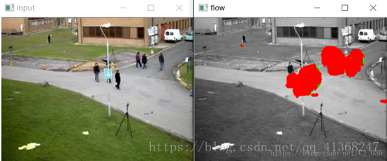
光流法检测运动物体基本原理是：给图像中每一个像素点赋予一个速度矢量，这就形成了一个图像运动场，在运动的一个特定时刻，图像上点与三维物体上点一一对应，这种对应关系可由投影关系得到，根据各个像素点的速度矢量特征，可以对图像进行动态分析。如果图像中没有运动物体，则光流矢量在整个图像区域是连续变化的。当图像中有运动物体时，目标和图像背景存在相对运动，运动物体所形成的速度矢量必然和邻域背景速度矢量不同，从而检测出运动物体及位置。采用光流法进行运动物体检测的问题主要在于大多数光流法计算耗时，实时性和实用性都较差。但是光流法的优点在于光流不仅携带了运动物体的运动信息，而且还携带了有关景物三维结构的丰富信息，它能够在不知道场景的任何信息的情况下，检测出运动对象。

对于视频监控系统来说，所用的图像基本都是摄像机静止状态下摄取得，所以对有实时性和准确性要求的系统来说，纯粹使用光流法来检测目标不太实际。更多的是利用光流计算方法与其它方法相结合来实现对目标检测和运动估计。

然而，在实际应用中，由于遮挡性、多光源、透明性和噪声等原因，使得光流场基本方程的灰度守恒假设条件不能满足，不能求解出正确的光流场，同时大多数的光流计算方法相当复杂，计算量巨大，不能满足实时的要求，因此，一般不被对精度和实时性要求比较高的监控系统所采用。

亮度恒定，就是同一点随着时间的变化，其亮度不会发生改变。这是基本光流法的假定（所有光流法变种都必须满足），用于得到光流法基本方程；
小运动，这个也必须满足，就是时间的变化不会引起位置的剧烈变化，这样灰度才能对位置求偏导（换句话说，小运动情况下我们才能用前后帧之间单位位置变化引起的灰度变化去近似灰度对位置的偏导数），这也是光流法不可或缺的假定；
空间一致，一个场景上邻近的点投影到图像上也是邻近点，且邻近点速度一致。这是Lucas-Kanade光流法特有的假定，因为光流法基本方程约束只有一个，而要求x，y方向的速度，有两个未知变量。我们假定特征点邻域内做相似运动，就可以连立n多个方程求取x，y方向的速度（n为特征点邻域总点数，包括该特征点）。

光流法用于目标跟踪的原理

对一个连续的视频帧序列进行处理；
针对每一个视频序列，利用一定的目标检测方法，检测可能出现的前景目标；
如果某一帧出现了前景目标，找到其具有代表性的关键特征点（可以随机产生，也可以利用角点来做特征点）；
对之后的任意两个相邻视频帧而言，寻找上一帧中出现的关键特征点在当前帧中的最佳位置，从而得到前景目标在当前帧中的位置坐标；
如此迭代进行，便可实现目标的跟踪；

由基本光流约束方程IxVx+IyVy+It=0可知，对于二维的运动场，单靠一个像素无法确定其运动矢量（Vx,Vy）；根据假设三，我们可以使用当前像素的邻域像素添加更多约束条件；如经典的Horn-Schunck光流法所加的运动平滑约束。同时，对于二维运动场，只需包含两条或以上边缘则可以解系统方程，因此在进行光流法时，先选择好跟踪的特征点，如harris角点。

光流场是运动场在二维图像上的投影，而光流就是在图像灰度模式下，像素点的运动矢量。光流法技术的核心就是求解出运动目标的光流，即速度。根据视觉感知原理，客观物体在空间上一般是相对连续运动的，在运动过程中，投射到传感器平面上的图像实际上也是连续变化的。为此可以假设:瞬时灰度值不变，即灰度不变性原理。由此可以得到光流基本方程，灰度对时间的变化率等于灰度的空间梯度与光流速度的点积。此时需要引入另外的约束条件，从不同的角度引入约束条件，导致了不同的光流分析方法。

Lucas-Kanada算法

Lucas-Kanada即L-K光流法最初于1981年提出，该算法假设在一个小的空间邻域内运动矢量保持恒定，使用加权最小二乘法估计光流。由于该算法应用于输入图像的一组点上时比较方便，因此被广泛应用于稀疏光流场，L-K算法的提出是基于以下三个假设：

亮度恒定不变。目标像素在不同帧间运动时外观上是保持不变的，对于灰度图像，假设在整个被跟踪期间，像素亮度不变；
时间连续或者运动是“小运动”。图像运动相对于时间来说比较缓慢，实际应用中指时间变化相对图像中运动比例要足够小，这样目标在相邻帧间的运动就比较小；
空间一致。同一场景中同一表面上的邻近点运动情况相似，且这些点在图像上的投影也在邻近区域。

对于假设条件：

亮度恒定，就是同一点随着时间的变化，其亮度不会发生改变。这是基本光流法的假定（所有光流法变种都必须满足），用于得到光流法基本方程；
小运动，这个也必须满足，就是时间的变化不会引起位置的剧烈变化，这样灰度才能对位置求偏导（换句话说，小运动情况下我们才能用前后帧之间单位位置变化引起的灰度变化去近似灰度对位置的偏导数），这也是光流法不可或缺的假定；
空间一致，一个场景上邻近的点投影到图像上也是邻近点，且邻近点速度一致。这是Lucas-Kanade光流法特有的假定，因为光流法基本方程约束只有一个，而要求x，y方向的速度，有两个未知变量。我们假定特征点邻域内做相似运动，就可以连立n多个方程求取x，y方向的速度（n为特征点邻域总点数，包括该特征点）。

对于方程求解：

多个方程求两个未知变量，又是线性方程，很容易就想到用最小二乘法，事实上opencv也是这么做的。其中，最小误差平方和为最优化指标。

对于前面说到了小运动这个假定，如果目标速度很快该怎么办呢？幸运的是多尺度能解决这个问题。首先，对每一帧建立一个高斯金字塔，最大尺度图片在最顶层，原始图片在底层。然后，从顶层开始估计下一帧所在位置，作为下一层的初始位置，沿着金字塔向下搜索，重复估计动作，直到到达金字塔的底层。这样搜索不仅可以解决大运动目标跟踪，也可以一定程度上解决孔径问题（相同大小的窗口能覆盖大尺度图片上尽量多的角点，而这些角点无法在原始图片上被覆盖）。

光流法国内外现状

对光流算法的研究，最早可追溯到二十世纪五十年代，Gibson和Wallach等学者提出的SFM（Structure From Motion）假设，即以心理学实验为基础，开创性的提出从二维平面的光流场可以恢复到三维空间运动参数和结构参数的假设，但该假设直到七十年代末才有ULLman等学者验证该假设。真正提出有效光流计算方法还归功于Horn和Schunck在1981年创造性地将二维速度场与灰度相联系，引入光流约束方程的算法，是光流算法发展的基石。光流算法发展至今不下几十种，其中许多是基于一阶时空梯度技术，其方法不仅效率高，且易于实现，总的深入分析可将光流算法分为四类。

（1）研究解决光流场计算的不适定问题的方法

在研究解决光流场计算不适定问题的方法的过程中，学者们提出了很多克服不适定问题的算法，例如Horn根据同一个运动物体的光流场具有连续、平滑的特点，即三维图像投影到二维图像上的光流变化也是平滑的，提出一个附加约束条件，将光流场的整体平滑约束转换为一个变分的问题；Tretiak和Nagel认为对光流场的计算属于一类微分问题，由于要涉及图像灰度时空导数计算，而提出了在二阶微分算子的基础上添加一个附加约束；Nagel提出为使附加的光滑性约束沿光流场梯度的垂直方向上变化率最小，导出了一种新的迭代算法；Wohu等人利用非线性平滑条件和局部约束来计算时变序列图像的光流场；Haralick等人通过将二维物体表面分割为若干个小平面，并假设小平面运动方向，速度近似，且在短时间内为常量，据此思想基础上得到了附件约束。国内复旦大学的吴立德教授对灰度时变图像光流场的理论进行过研究并提出了多通道方法。

（2）研究光流场计算的快速算法

在光流算法快速算法研究中，Braillon提出一种光流模型检测障碍物的方法，该方法是为摄像机建立经典的针孔模型，并在针孔模型上建光流模型，并不需要计算完整的光流场；Valentinotti在并行的DSP系统上实现了基于相位的光流算法，对128×128和64×64图像序列实现了快速处理；Andres Bruhn等人在对光流计算时引入了多尺度分析，提高了计算的效率；昌猛等人在Horn-Schunck算法的递归方程的基础上添加了一个惯性因子，性能不降低，然而收敛时间缩短了1/2-1/3，也极大的提高了计算效率。

（3）研究光流场计算基本公式的不连续性

在光流场计算基本公式导出过程中由于利用泰勒级数展开，实际上认为图像灰度以及亮度场变化都是连续的。然而，实际景物各个独立的表面就使光流的速度场成为非连续的，因此当光流场计算基本公式出现不连续时，是个值得讨论的问题，日本学者 Mukauwa考虑光流场计算基本等式应用泰勒级数展开后，实际上是不连续的，他引入了一个修正因子q后，很好的解决了不连续性的问题。

（4）研究直线和曲线的光流场计算技术

光流场的计算是计算机视觉的重要组成部分，主要是通过二维空间的光流场恢复重建三维物体的运动和结构。一般来说，用单个像素点来表示光流场显然不合适，通过抽象层次手工劳动提高像素点将更有利于进行图像处理和分析。例如，Allmen就是通过定义时空表面流为时空表面光流的延伸，认为轮廓线移动时，它们在平面上的投影也相对移动，利用它们在时空表面流与空间流曲线来计算光流场；Kumar提出一种可以很好的保留边界信息的新的计算光流场的曲线方法，其计算结果和理论分析非常吻合；Park利用轮廓线曲率信息去估算轮廓线的运动。

光流法意义

将三维空间中的目标和场景对应于二维图像平面运动时，他们在二维图像平面的投影就形成了运动，这种运动以图像平面亮度模式表现出来的流动就称为光流。光流法是对运动序列图像进行分析的一个重要方法，光流不仅包含图像中目标的运动信息，而且包含了三维物理结构的丰富信息，因此可用来确定目标的运动情况以及反映图像其它等信息。

基于光流可以实现在军事航天、交通监管、信息科学、气象、医学等多个领域的重要应用。例如利用光流场可以非常有效的对图像目标进行检测和分割，这对地对空导弹火控系统的精确制导，自动飞行器精确导航与着陆，战场的动态分析，军事侦察的航天或卫星图片的自动分析系统，医学上异常器官细胞的分析与诊断系统，气象中对云图的运动分析，城市交通的车流量进行监管都具有重要价值。

当前对于光流法的研究主要有两个方向：一是研究在固有硬件平台基础上实现现有算法，二是研究新的算法。光流算法的主要目的就是基于序列图像实现对光流场的可靠、快速、精确以及鲁棒性的估计。然而，由于图像序列目标的特性、场景中照明，光源的变化、运动的速度以及噪声的影响等多种因素影响着光流算法的有效性。尽管近几十年来，国内外学者提出了各种各样的光流场的算法，然而，建立可靠的光流算法模型仍然面临很大的挑战。开展研究光流算法涉及多个学科领域的理论和技术，如图像处理、计算机科学、模式识别、矩阵分析、优化理论等。对这一研究的发展不仅拓宽了这些领域的理论基础和技术研究范畴，而且为这些理论和技术的应用打开一扇新的窗口。

稠密光流与稀疏光流

除了根据原理的不同来区分光流法外，还可以根据所形成的光流场中二维矢量的疏密程度将光流法分为稠密光流与稀疏光流两种。

稠密光流

稠密光流是一种针对图像或指定的某一片区域进行逐点匹配的图像配准方法，它计算图像上所有的点的偏移量，从而形成一个稠密的光流场。通过这个稠密的光流场，可以进行像素级别的图像配准。

Horn-Schunck算法以及基于区域匹配的大多数光流法都属于稠密光流的范畴。

基于区域匹配方法生成稠密光流场

由于光流矢量稠密，所以其配准后的效果也明显优于稀疏光流配准的效果。但是其副作用也是明显的，由于要计算每个点的偏移量，其计算量也明显较大，时效性较差。

稀疏光流

与稠密光流相反，稀疏光流并不对图像的每个像素点进行逐点计算。它通常需要指定一组点进行跟踪，这组点最好具有某种明显的特性，例如Harris角点等，那么跟踪就会相对稳定和可靠。稀疏跟踪的计算开销比稠密跟踪小得多。

基于特征的匹配方法是典型的属于稀疏光流的算法。

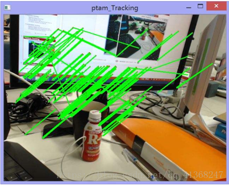
基于特征匹配方法生成稀疏光流场

HALCON光流法算子

optical_flow_mg

optical_flow_mg — Compute the optical flow between two images.	optical_flow_mg：计算两幅图像之间的光流。
optical_flow_mg(ImageT1, ImageT2 : VectorField : Algorithm, SmoothingSigma, IntegrationSigma, FlowSmoothness, GradientConstancy, MGParamName, MGParamValue : )	optical_flow_mg(ImageT1, ImageT2 : VectorField : Algorithm, SmoothingSigma, IntegrationSigma, FlowSmoothness, GradientConstancy, MGParamName, MGParamValue : )
optical_flow_mg computes the optical flow between two images. The optical flow represents information about the movement between two consecutive images of a monocular image sequence. The movement in the images can be caused by objects that move in the world or by a movement of the camera (or both) between the acquisition of the two images. The projection of these 3D movements into the 2D image plane is called the optical flow.	optical_flow_mg计算两幅图像之间的光流。光流表示单目图像序列中两个连续图像之间运动的信息。图像中的运动可以由物体在世界上的运动引起，也可以由相机(或两者)在获取两幅图像之间的运动引起。这些三维运动在二维图像平面上的投影称为光流。
The two consecutive images of the image sequence are passed in ImageT1 and ImageT2. The computed optical flow is returned in VectorField. The vectors in the vector field VectorField represent the movement in the image plane between ImageT1 andImageT2. The point in ImageT2 that corresponds to the point (r,c) in ImageT1 is given by (r',c') = (r+u(r,c),c+v(r,c)), where u(r,c) and v(r,c) denote the value of the row and column components of the vector field image VectorField at the point (r,c).	图像序列的两个连续图像传递到ImageT1和ImageT2。计算得到的光流返回到VectorField。VectorField向量场中的向量表示ImageT1和ImageT2之间的图像平面上的运动。ImageT2中对应于ImageT1中(r,c)点的点由(r'，c') = (r+u(r,c)，c+v(r,c))给出，其中u(r,c)和v(r,c)表示VectorField的行和列分量在点(r,c)处的值。
The parameter Algorithm allows the selection of three different algorithms for computing the optical flow. All three algorithms are implemented by using multigrid solvers to ensure an efficient solution of the underlying partial differential equations.	参数Algorithm允许选择三种不同的算法来计算光流。这三种算法都是通过使用多重网格求解器来实现的，以确保底层偏微分方程的有效解。
For Algorithm = 'fdrig', the method proposed by Brox, Bruhn, Papenberg, and Weickert is used. This approach is flow-driven, robust, isotropic, and uses a gradient constancy term. For Algorithm = 'ddraw', a robust variant of the method proposed by Nagel and Enkelmann is used. This approach is data-driven, robust, anisotropic, and uses warping (in contrast to the original approach). For Algorithm = 'clg' the combined local-global method proposed by Bruhn, Weickert, Feddern, Kohlberger, and Schnörr is used.	对于Algorithm = 'fdrig'，使用了Brox、Bruhn、Papenberg和Weickert提出的方法。该方法是流驱动的、鲁棒的、各向同性的、并使用了梯度恒常性。对于Algorithm = 'ddraw'，使用了Nagel和Enkelmann提出方法的鲁棒变体。这种方法是数据驱动的、鲁棒的、各向异性的，并且使用了扭曲(与原始方法相反)。对于Algorithm = 'clg'采用了Bruhn、Weickert、Feddern、Kohlberger和Schnorr提出的局部-全局结合方法。
In all three algorithms, the input images can first be smoothed by a Gaussian filter with a standard deviation of SmoothingSigma (see derivate_gauss).	在这三种算法中，输入图像都首先通过一个标准偏差为SmoothingSigma的高斯滤波器进行平滑(参见derivate_gauss)。
All three approaches are variational approaches that compute the optical flow as the minimizer of a suitable energy functional. In general, the energy functionals have the following form: where w=(u,v,1) is the optical flow vector field to be determined (with a time step of 1 in the third coordinate). The image sequence is regarded as a continuous function f(x), where x=(r,c,t) and (r,c) denotes the position and t the time. Furthermore, denotes the data term, while denotes the smoothness term, and α is a regularization parameter that determines the smoothness of the solution. The regularization parameter α is passed in FlowSmoothness. While the data term encodes assumptions about the constancy of the object features in consecutive images, e.g., the constancy of the gray values or the constancy of the first spatial derivative of the gray values, the smoothness term encodes assumptions about the (piecewise) smoothness of the solution, i.e., the smoothness of the vector field to be determined.	这三种方法都是变分方法，即计算光流作为合适能量泛函的最小值。一般来说，能量泛函的形式如下：其中w=(u,v,1)为待确定光流向量场(第三坐标时间步长为1)。将图像序列视为连续函数f(x)，其中x=(r,c,t)，(r,c)表示位置，t表示时间。其中，为数据项，为平滑项，α为决定解平滑程度的正则化参数。正则化参数α由FlowSmoothness传递。数据项对连续图像中目标特征的稳定性进行假设，如灰度值的恒常性或灰度值的一阶空间导数的恒常性，而平滑项对解的(分段)平滑性进行假设，即待确定向量场的平滑度。
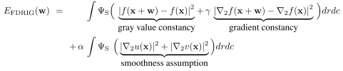
The FDRIG algorithm is based on the minimization of an energy functional that contains the following assumptions: Constancy of the gray values: It is assumed that corresponding pixels in consecutive images of an image sequence have the same gray value, i.e., that f(r+u,c+v,t+1) = f(r,c,t). This can be written more compactly as f(x+w) = f(x) using vector notation. Constancy of the spatial gray value derivatives: It is assumed that corresponding pixels in consecutive images of an image sequence additionally have the same spatial gray value derivatives, i.e, that also holds, where . This can be written more compactly as . In contrast to the gray value constancy, the gradient constancy has the advantage that it is invariant to additive global illumination changes. Large displacements: It is assumed that large displacements, i.e., displacements larger than one pixel, occur. Under this assumption, it makes sense to consciously abstain from using the linearization of the constancy assumptions in the model that is typically proposed in the literature. Statistical robustness in the data term: To reduce the influence of outliers, i.e., points that violate the constancy assumptions, they are penalized in a statistically robust manner, i.e., the customary non-robust quadratical penalization is replaced by a linear penalization via , where is a fixed regularization constant. Preservation of discontinuities in the flow field I: The solution is assumed to be piecewise smooth. While the actual smoothness is achieved by penalizing the first derivatives of the flow , the use of a statistically robust (linear) penalty function with provides the desired preservation of edges in the movement in the flow field to be determined. This type of smoothness term is called flow-driven and isotropic. Taking into account all of the above assumptions, the energy functional of the FDRIG algorithm can be written as： Here, α is the regularization parameter passed in FlowSmoothness, whileγis the gradient constancy weight passed in GradientConstancy. These two parameters, which constitute the model parameters of the FDRIG algorithm, are described in more detail below.	FDRIG算法基于能量泛函的最小化，其中包含以下假设：灰度值的恒常性：假设图像序列的连续图像中对应像素具有相同的灰度值，即f(r+u,c+v,t+1) = f(r,c,t)，可以更简洁地用向量表示法写成f(x+w) = f(x)。空间灰度值导数的恒常性：假设图像序列的连续图像中对应的像素具有相同的空间灰度值导数，如也成立，其中。可以更简洁地写成。与灰度值恒常性相比，梯度恒常性的优点是不受全局光照变化的影响。大位移：假定大位移，即发生大于一个像素的位移。在这种假设下，有意识地避免在模型中使用通常在文献中提出的恒常性假设的线性化是有意义的。数据项的统计鲁棒性：减少异常值的影响，即违反恒常性假设的点，会以统计上鲁棒方式受到惩罚，即用线性惩罚代替传统的非鲁棒二次惩罚，其中是固定的正则化常数。在流场I中不连续性的保持：假设解是分段光滑的。虽然实际的平滑度是通过惩罚流的一阶导数来实现的，但是使用统计上的鲁棒(线性)惩罚函数（）可以在待确定的流场中提供所需的边缘保存。这种类型的平滑项称为流驱动和各向同性。考虑上述假设,FDRIG算法的能量函数可以写成：其中，α为FlowSmoothness传递的正则化参数，γ为GradientConstancy传递的梯度恒常性权重。这两个参数构成了FDRIG算法的模型参数，下面将对它们进行更详细的描述。
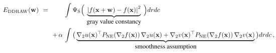
The DDRAW algorithm is based on the minimization of an energy functional that contains the following assumptions: Constancy of the gray values: It is assumed that corresponding pixels in consecutive images of an image sequence have the same gray value, i.e., that f(x+w) = f(x). Large displacements: It is assumed that large displacements, i.e., displacements larger than one pixel, occur. Under this assumption, it makes sense to consciously abstain from using the linearization of the constancy assumptions in the model that is typically proposed in the literature. Statistical robustness in the data term: To reduce the influence of outliers, i.e., points that violate the constancy assumptions, they are penalized in a statistically robust manner, i.e., the customary non-robust quadratical penalization is replaced by a linear penalization via , where is a fixed regularization constant. Preservation of discontinuities in the flow field II: The solution is assumed to be piecewise smooth. In contrast to the FDRIG algorithm, which allows discontinuities everywhere, the DDRAW algorithm only allows discontinuities at the edges in the original image. Here, the local smoothness is controlled in such a way that the flow field is sharp across image edges, while it is smooth along the image edges. This type of smoothness term is called data-driven and anisotropic. All assumptions of the DDRAW algorithm can be combined into the following energy functional: where is a normalized projection matrix orthogonal to , for which holds. This matrix ensures that the smoothness of the flow field is only assumed along the image edges. In contrast, no assumption is made with respect to the smoothness across the image edges, resulting in the fact that discontinuities in the solution may occur across the image edges. In this respect, serves as a regularization parameter that prevents the projection matrix from becoming singular. In contrast to the FDRIG algorithm, there is only one model parameter for the DDRAW algorithm: the regularization parameter α. As mentioned above, α is described in more detail below.	DDRAW算法基于能量泛函最小化，其中包含以下假设：灰度值的恒常性：假设图像序列的连续图像中对应像素具有相同的灰度值，即f(x+w) = f(x)。大位移：假定大位移，即发生大于一个像素的位移。在这种假设下，有意识地避免在模型中使用通常在文献中提出的恒常性假设的线性化是有意义的。数据项的统计鲁棒性：减少异常值的影响，即违反恒常性假设的点，会以统计上鲁棒方式受到惩罚，即用线性惩罚代替传统的非鲁棒二次惩罚，其中是一个固定的正则化常数。流场中不连续性的保持II：假设解是分段光滑的。FDRIG算法允许任何地方都存在不连续。与FDRIG算法相反，DDRAW算法只允许原始图像边缘的不连续点。流场在图像边缘是尖锐的，因此控制局部平滑的方法是在图像边缘平滑流场。这种类型的平滑项称为数据驱动和各向异性。 DDRAW算法的所有假设可以合并为以下能量泛函：是正交于的归一化投影矩阵，对于成立。该矩阵保证了流场的光滑性仅沿图像边缘假设。相反，没有对图像边缘的平滑度做任何假设，从而导致解决方案中的不连续可能发生在图像边缘。在这方面，作为一个正则化参数，防止投影矩阵成为奇异的。与FDRIG算法相比，DDRAW算法只有一个模型参数：正则化参数α。如前所述，α在下面更详细地描述。
As for the two approaches described above, the CLG algorithm uses certain assumptions: Constancy of the gray values: It is assumed that corresponding pixels in consecutive images of an image sequence have the same gray value, i.e., that f(x+w) = f(x). Small displacements: In contrast to the two approaches above, it is assumed that only small displacements can occur, i.e., displacements in the order of a few pixels. This facilitates a linearization of the constancy assumptions in the model, and leads to the approximation , i.e., should hold. Here, denotes the gradient in the spatial as well as the temporal domain. Local constancy of the solution: Furthermore, it is assumed that the flow field to be computed is locally constant. This facilitates the integration of the image data in the data term over the respective neighborhood of each pixel. This, in turn, increases the robustness of the algorithm against noise. Mathematically, this can be achieved by reformulating the quadratic data term as. By performing a local Gaussian-weighted integration over a neighborhood specified by the ρ (passed in IntegrationSigma), the following data term is obtained: . Here, denotes a convolution of the 3x3 matrix with a Gaussian filter with a standard deviation of ρ (see derivate_gauss). General smoothness of the flow field: Finally, the solution is assumed to be smooth everywhere in the image. This particular type of smoothness term is called homogeneous. All of the above assumptions can be combined into the following energy functional:	对比上述两种方法，CLG算法使用了一定的假设：灰度值的恒常性：假设图像序列的连续图像中对应像素具有相同的灰度值，即f(x+w) = f(x)。小位移：与上述两种方法相比，CLG假设只有小位移才会发生，即位移按几个像素的顺序排列。这有利于模型中恒常性假设的线性化，并导致近似，即应该成立。表示空间和时间域的梯度。解的局部恒常性：此外，假定要计算的流场是局部恒常的。这有助于将数据项中的图像数据集成到每个像素的相应邻域上。这进而提高了算法对噪声的鲁棒性。从数学上讲，这可以通过重新制定二次数据项来实现。通过对指定的邻域进行局部高斯加权积分，得到以下数据项：。式中，为3x3矩阵与高斯滤波器的卷积，其标准差为ρ(见derivate_gauss)。流场的一般光滑性：最后，假设解在图像中处处光滑。这种特殊类型的平滑项称为齐次的。上述所有假设可以合并为以下能量泛函：对应的模型参数是正则化参数α和积分尺度ρ(IntegrationSigma)，它决定了要对数据项进行积分的邻域的大小。下面将更详细地描述这两个参数。
To compute the optical flow vector field for two consecutive images of an image sequence with the FDRIG, DDRAW, or CLG algorithm, the solution that best fulfills the assumptions of the respective algorithm must be determined. From a mathematical point of view, this means that a minimization of the above energy functionals should be performed. For the FDRIG and DDRAW algorithms, so called coarse-to-fine warping strategies play an important role in this minimization, because they enable the calculation of large displacements. Thus, they are a suitable means to handle the omission of the linearization of the constancy assumptions numerically in these two approaches. To calculate large displacements, coarse-to-fine warping strategies use two concepts that are closely interlocked: The successive refinement of the problem (coarse-to-fine) and the successive compensation of the current image pair by already computed displacements (warping). Algorithmically, such coarse-to-fine warping strategies can be described as follows: 1. First, both images of the current image pair are zoomed down to a very coarse resolution level. 2. Then, the optical flow vector field is computed on this coarse resolution. 3. The vector field is required on the next resolution level: It is applied there to the second image of the image sequence, i.e., the problem on the finer resolution level is compensated by the already computed optical flow field. This step is also known as warping. 4. The modified problem (difference problem) is now solved on the finer resolution level, i.e., the optical flow vector field is computed there. 5. The steps 3-4 are repeated until the finest resolution level is reached. 6. The final result is computed by adding up the vector fields from all resolution levels. This incremental computation of the optical flow vector field has the following advantage: While the coarse-to-fine strategy ensures that the displacements on the finest resolution level are very small, the warping strategy ensures that the displacements remain small for the incremental displacements (optical flow vector fields of the difference problems). Since small displacements can be computed much more accurately than larger displacements, the accuracy of the results typically increases significantly by using such a coarse-to-fine warping strategy.	要用FDRIG、DDRAW或CLG算法计算图像序列中连续两幅图像的光流向量场，必须确定最能满足各自算法假设的解。从数学的角度来看，这意味着应该执行上述能量泛函的最小化。对于FDRIG和DDRAW算法来说，所谓的“粗到细”的扭曲策略在这种最小化中扮演着重要的角色，因为它们能够计算大位移。因此，这两种方法在数值上都能较好地解决恒常性假设线性化的不足。为了计算大位移，“粗到细”的扭曲策略使用了两个紧密相连的概念：问题的连续细化(粗到细)和通过已计算的位移对当前图像对的连续补偿(扭曲)。算法上，这种由“粗到细”的扭曲策略可以描述为： 1. 首先，将当前图像对的两个图像都缩小到非常粗的分辨率级别； 2. 然后，在此粗分辨率基础上计算光流向量场； 3. 向量场是下一分辨率层所需要的：它应用于图像序列的第二幅图像，即在较细分辨率水平上的问题是由已计算的光流向量场补偿。这一步也被称为扭曲； 4. 修改后的问题(差分问题)现在在较细的分辨率级别上得到解决，即计算了光流向量场； 5. 重复上述步骤3～4，直到达到最佳分辨率； 6. 最后的结果是通过将所有分辨率级别的向量场相加来计算的。这个增量计算光流向量场具有以下优势：虽然由粗到细的策略确保在最细分辨率水平上的位移非常小，翘曲策略保证了增量位移保持较小的位移(光流向量场的区别问题)。由于小位移的计算要比大位移精确得多，因此使用这种由粗到细的扭曲策略，结果的精度通常会显著提高。
However, instead of having to solve a single correspondence problem, an entire hierarchy of these problems must now be solved. For the CLG algorithm, such a coarse-to-fine warping strategy is unnecessary since the model already assumes small displacements. The maximum number of resolution levels (warping levels), the resolution ratio between two consecutive resolution levels, as well as the finest resolution level can be specified for the FDRIG as well as the DDRAW algorithm. Details can be found below. The minimization of functionals is mathematically very closely related to the minimization of functions: Like the fact that the zero crossing of the first derivative is a necessary condition for the minimum of a function, the fulfillment of the so called Euler-Lagrange equations is a necessary condition for the minimizing function of a functional (the minimizing function corresponds to the desired optical flow vector field in this case). The Euler-Lagrange equations are partial differential equations. By discretizing these Euler-Lagrange equations using finite differences, large sparse nonlinear equation systems result for the FDRIG and DDRAW algorithms. Because coarse-to-fine warping strategies are used, such an equation system must be solved for each resolution level, i.e., for each warping level. For the CLG algorithm, a single sparse linear equation system must be solved.	然而，现在必须解决这些问题的整个层次结构，而不是单个的对应问题。对于CLG算法，这种由粗到细的扭曲策略是不必要的，因为模型已经假定了较小的位移。可以为FDRIG和DDRAW算法指定最大分辨率级别(扭曲级别)、两个连续分辨率级别之间的分辨率比以及最佳分辨率级别。详情如下。泛函的极小化是非常密切相关的数学函数的最小化：事实上一阶导数的零交叉是函数最小化的必要条件，是实现所谓的欧拉方程的最小化函数功能的必要条件(在这种情况下最小化函数对应于所需的光流向量场)。欧拉-拉格朗日方程是偏微分方程。通过对这些欧拉-拉格朗日方程进行有限差分离散化，得到了大稀疏非线性方程组的FDRIG和DDRAW算法结果。由于采用了由粗到细的扭曲策略，因此必须针对每个分辨率级别求解这样一个方程组，即每一个扭曲水平。对于CLG算法，必须求解一个稀疏线性方程组。
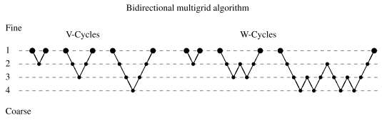
To ensure that the above nonlinear equation systems can be solved efficiently, the FDRIG and DDRAW use bidirectional multigrid methods. From a numerical point of view, these strategies are among the fastest methods for solving large linear and nonlinear equation systems. In contrast to conventional nonhierarchical iterative methods, e.g., the different linear and nonlinear Gauss-Seidel variants, the multigrid methods have the advantage that corrections to the solution can be determined efficiently on coarser resolution levels. This, in turn, leads to a significantly faster convergence. The basic idea of multigrid methods additionally consists of hierarchically computing these correction steps, i.e., the computation of the error on a coarser resolution level itself uses the same strategy and efficiently computes its error (i.e., the error of the error) by correction steps on an even coarser resolution level. Depending on whether one or two error correction steps are performed per cycle, a so called V or W cycle is obtained. The corresponding strategies for stepping through the resolution hierarchy are as follows for two to four resolution levels: Here, iterations on the original problem are denoted by large markers, while small markers denote iterations on error correction problems.	为了保证上述非线性方程组的有效求解，FDRIG和DDRAW采用双向多重网格方法。从数值的角度来看，这些策略是求解大型线性和非线性方程组的最快方法之一。与传统的非层次迭代方法相比，如不同的线性和非线性Gauss-Seidel变分，多重网格方法的优点是可以在较粗的分辨率水平上有效地确定解的修正。这进而导致了显著的更快的收敛。多网格方法的基本思想还包括分层计算这些修正步骤，即在较粗分辨率级别上计算误差本身使用相同的策略，并能通过更粗的分辨率水平修正步骤上的误差有效地计算其误差(即误差的误差)。根据每个周期执行一个或两个纠错步骤，可以得到所谓的V或W周期。对于2至4个分辨率级别，通过分辨率层次结构的相应策略如下：这里，原始问题的迭代用大标记表示，小标记表示纠错问题的迭代。
Algorithmically, a correction cycle can be described as follows: 1. In the first step, several (few) iterations using an interative linear or nonlinear basic solver are performed (e.g., a variant of the Gauss-Seidel solver). This step is called pre-relaxation step. 2. In the second step, the current error is computed to correct the current solution (the solution after step 1). For efficiency reasons, the error is calculated on a coarser resolution level. This step, which can be performed iteratively several times, is called coarse grid correction step. 3. In a final step, again several (few) iterations using the interative linear or nonlinear basic solver of step 1 are performed. This step is called post-relaxation step.	算法上，修正周期可以描述为： 1. 在第一步中，使用交互式线性或非线性基本求解器(例如，Gauss-Seidel求解器的一个变体)执行几个(少数)迭代。这个步骤叫做预松弛步骤； 2. 在第二步中，计算当前误差来修正当前解(第一步后的解)。为了提高效率，计算误差的分辨率较粗。此步骤可迭代执行多次，称为粗网格校正步骤； 3. 在最后一个步骤中，再次使用第1步的交互式线性或非线性基本求解器进行几次迭代。这个步骤叫做后松弛步骤。
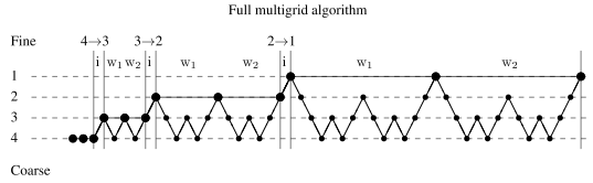
In addition, the solution can be initialized in a hierarchical manner. Starting from a very coarse variant of the original (non)linear equation system, the solution is successively refined. To do so, interpolated solutions of coarser variants of the equation system are used as the initialization of the next finer variant. On each resolution level itself, the V or W cycles described above are used to efficiently solve the (non)linear equation system on that resolution level. The corresponding multigrid methods are called full multigrid methods in the literature. The full multigrid algorithm can be visualized as follows: This example represents a full multigrid algorithm that uses two W correction cycles per resolution level of the hierarchical initialization. The interpolation steps of the solution from one resolution level to the next are denoted by i and the two W correction cycles by W1 and W2. Iterations on the original problem are denoted by large markers, while small markers denote iterations on error correction problems.	此外，可以以分层的方式初始化解决方案。从原始(非线性)方程系统的一个非常粗糙的变体开始，解被不断地细化。为了做到这一点，将方程系统中较粗变量的插值解作为下一个较细变量的初始化。在每个分辨率级别上，上面描述的V或W循环用于在该分辨率级别上有效地求解(非线性)方程组。相应的多重网格方法在文献中称为全多重网格方法。完整的多重网格算法可以可视化如下：这个例子代表了一个完整的多重网格算法，它使用了分层初始化的每个分辨率级别上的两个W校正周期。从一个分辨率级到下一个分辨率级的插值步骤用i和两个W的校正周期W1、W2表示。原始问题的迭代用大标记表示，小标记表示纠错问题的迭代。
In the multigrid implementation of the FDRIG, DDRAW, and CLG algorithm, the following parameters can be set: whether a hierarchical initialization is performed; the number of coarse grid correction steps; the maximum number of correction levels (resolution levels); the number of pre-relaxation steps; the number of post-relaxation steps. These parameters are described in more detail below. The basic solver for the FDRIG algorithm is a point-coupled fixed-point variant of the linear Gauss-Seidel algorithm. The basic solver for the DDRAW algorithm is an alternating line-coupled fixed-point variant of the same type. The number of fixed-point steps can be specified for both algorithms with a further parameter. The basic solver for the CLG algorithm is a point-coupled linear Gauss-Seidel algorithm. The transfer of the data between the different resolution levels is performed by area-based interpolation and area-based averaging, respectively.	在FDRIG、DDRAW和CLG算法的多网格实现中，可以设置以下参数：是否执行分层初始化；粗网格校正步数；校正水平的最大次数(分辨率水平)；预松弛步骤数；后松弛步骤数。下面将更详细地描述这些参数。 FDRIG算法的基本求解器是线性Gauss-Seidel算法的点耦合定点变体。DDRAW算法的基本求解器是同一类型的交替线耦合定点变量。可以使用进一步的参数为这两种算法指定定点步骤的数量。CLG算法的基本求解器是点耦合线性Gauss-Seidel算法。在不同分辨率水平之间的数据传输分别采用基于区域的插值和基于区域的平均方法。
After the algorithms have been described, the effects of the individual parameters are discussed in the following.	在描述了算法之后，下面讨论各个参数的影响。
The input images, along with their domains (regions of interest) are passed in ImageT1 and ImageT2. The computation of the optical flow vector field VectorField is performed on the smallest surrounding rectangle of the intersection of the domains of ImageT1 and ImageT2. The domain of VectorField is the intersection of the two domains. Hence, by specifying reduced domains for ImageT1 and ImageT2, the processing can be focused and runtime can potentially be saved. It should be noted, however, that all methods compute a global solution of the optical flow. In particular, it follows that the solution on a reduced domain need not (and cannot) be identical to the resolution on the full domain restricted to the reduced domain.	输入图像及其域(感兴趣区域)传递到ImageT1和ImageT2。在ImageT1和ImageT2区域交集的最小外接矩形上计算光流向量场VectorField。VectorField的域是这两个域的交集。因此，通过指定ImageT1和ImageT2的简化域，可以专注处理，并可能节约运行时。但是，需要注意的是，所有方法都计算光流的全局解。特别是，可以得出结论，在简约域上的解决方案不必(也不可能)与在全域上的解决方案相同(全域上的解决方案仅限于简约域)。
SmoothingSigma specifies the standard deviation of the Gaussian kernel that is used to smooth both input images. The larger the value of SmoothingSigma, the larger the low-pass effect of the Gaussian kernel, i.e., the smoother the preprocessed image. Usually,SmoothingSigma = 0.8 is a suitable choice. However, other values in the interval [0,2] are also possible. Larger standard deviations should only be considered if the input images are very noisy. It should be noted that larger values of SmoothingSigma lead to slightly longer execution times.	SmoothingSigma指定用于平滑两个输入图像的Gaussian核的标准差。SmoothingSigma越大，Gaussian核的低通(low-pass)效应越大，即预处理后的图像越平滑。通常，SmoothingSigma = 0.8是一个合适的选择。然而，区间[0,2]中的其他值也是可能的。只有在输入图像噪声较大时才应考虑较大的标准差。应该注意的是，SmoothingSigma值越大，执行时间越长。
IntegrationSigma specifies the standard deviation ρ of the Gaussian kernel Gρ that is used for the local integration of the neighborhood information of the data term. This parameter is used only in the CLG algorithm and has no effect on the other two algorithms. Usually, IntegrationSigma = 1.0 is a suitable choice. However, other values in the interval [0,3] are also possible. Larger standard deviations should only be considered if the input images are very noisy. It should be noted that larger values of IntegrationSigmalead to slightly longer execution times.	IntegrationSigma指定用于对数据项的邻域信息进行局部积分的Gaussian核Gρ的标准差ρ。该参数仅在CLG算法中使用，对其他两种算法没有影响。通常，IntegrationSigma = 1.0是一个合适的选择。然而，区间[0,3]中的其他值也是可能的。只有在输入图像噪声较大时才应考虑较大的标准差。应该注意的是，较大的IntegrationSigmalead值会使执行时间稍微长一些。
FlowSmoothness specifies the weight α of the smoothness term with respect to the data term. The larger the value of FlowSmoothness, the smoother the computed optical flow field. It should be noted that choosing FlowSmoothness too small can lead to unusable results, even though statistically robust penalty functions are used, in particular if the warping strategy needs to predict too much information outside of the image. For byte images with a gray value range of [0,255], values of FlowSmoothness around 20 for the flow-driven FDRIG algorithm and around 1000 for the data-driven DDRAW algorithm and the homogeneous CLG algorithm typically yield good results.	flow smooth指定平滑项相对于数据项的权重α。FlowSmoothness越大，计算得到的光流场越光滑。需要注意的是，选择过小的FlowSmoothness可能会导致不可用的结果，即使使用了统计上健壮的惩罚函数，特别是当扭曲策略需要预测太多图像之外的信息时。对于灰度值范围为[0 255]的字节图像，流驱动的FDRIG算法的FlowSmoothness在20左右，数据驱动的DDRAW算法和齐次CLG算法的FlowSmoothness在1000左右，通常会得到很好的结果。
GradientConstancy specifies the weight γ of the gradient constancy with respect to the gray value constancy. This parameter is used only in the FDRIG algorithm. For the other two algorithms, it does not influence the results. For byte images with a gray value range of [0,255], a value of GradientConstancy = 5 is typically a good choice, since then both constancy assumptions are used to the same extent. For large changes in illumination, however, significantly larger values of GradientConstancy may be necessary to achieve good results. It should be noted that for large values of the gradient constancy weight the smoothness parameter FlowSmoothness must also be chosen larger.	GradientConstancy指定梯度恒常性相对于灰度值恒常性的权重γ。这个参数只在FDRIG算法中使用。对于另外两种算法，它不影响结果。对于灰度值范围为[0,255]的字节图像，GradientConstancy = 5通常是一个不错的选择，因为这两个恒常性假设在同一程度上使用。然而，对于光照变化较大的情况，可能需要显著增大的GradientConstancy值才能获得较好结果。需要注意的是，对于梯度恒常性权值较大的情况，还必须选择更大的平滑度参数FlowSmoothness。
The parameters of the multigrid solver and for the coarse-to-fine warping strategy can be specified with the generic parameters MGParamName and MGParamValue. Usually, it suffices to use one of the four default parameter sets via MGParamName = 'default_parameters'and MGParamValue = 'very_accurate', 'accurate', 'fast_accurate', or 'fast'. The default parameter sets are described below. If the parameters should be specified individually, MGParamName and MGParamValue must be set to tuples of the same length. The values corresponding to the parameters specified in MGParamName must be specified at the corresponding position in MGParamValue.	多网格求解器的参数以及由粗到细的扭曲策略可以用通用参数MGParamName和MGParamValue来指定。通常，通过MGParamName = 'default_parameters'和MGParamValue = 'very_accurate'、'accurate'、'fast_accurate'或'fast'，使用四个默认参数集中的一个就足够了。下面将描述缺省参数集。如果应该单独指定参数，则必须将MGParamName和MGParamValue设置为相同长度的元组。与MGParamName中指定的参数对应的值必须在MGParamValue中对应的位置指定。
MGParamName = 'warp_zoom_factor' can be used to specify the resolution ratio between two consecutive warping levels in the coarse-to-fine warping hierarchy. 'warp_zoom_factor' must be selected from the open interval (0,1). For performance reasons,'warp_zoom_factor' is typically set to 0.5, i.e., the number of pixels is halved in each direction for each coarser warping level. This leads to an increase of 33% in the calculations that need to be performed with respect to an algorithm that does not use warping. Values for'warp_zoom_factor' close to 1 can lead to slightly better results. However, they require a disproportionately larger computation time, e.g., 426% for 'warp_zoom_factor' = 0.9.	MGParamName = 'warp_zoom_factor'可用于指定粗到细的扭曲层次结构中两个连续扭曲级别之间的分辨率比率。必须从开区间(0,1)中选择'warp_zoom_factor'。出于性能原因，'warp_zoom_factor'通常设置为0.5，即对于每个较粗的扭曲级别，每个方向上的像素数减半。对于不使用扭曲的算法，这将导致需要执行的计算增加33%。'warp_zoom_factor'的值接近1时，结果会稍微好一些。但是，它们需要更多的计算时间，例如，对于'warp_zoom_factor' = 0.9，需要426%的计算时间。
MGParamName = 'warp_levels' can be used to restrict the warping hierarchy to a maximum number of levels. For 'warp_levels' = 0, the largest possible number of levels is used. If the image size does not allow to use the specified number of levels (taking the resolution ratio 'warp_zoom_factor' into account), the largest possible number of levels is used. Usually, 'warp_levels' should be set to 0.	MGParamName = 'warp_levels'可用于将扭曲层次结构限制为最大的层次数量。对于'warp_levels' = 0，使用尽可能多的级别。如果图像大小不允许使用指定数量的级别(考虑到分辨率'warp_zoom_factor')，则使用尽可能多的级别。通常，'warp_levels'应该设置为0。
MGParamName = 'warp_last_level' can be used to specify the number of warping levels for which the flow increment should no longer be computed. Usually, 'warp_last_level' is set to 1 or 2, i.e., a flow increment is computed for each warping level, or the finest warping level is skipped in the computation. Since in the latter case the computation is performed on an image of half the resolution of the original image, the gained computation time can be used to compute a more accurate solution, e.g., by using a full multigrid algorithm with additional iterations. The more accurate solution is then interpolated to the full resolution.	MGParamName = 'warp_last_level'可用于指定不再计算流增量的扭曲水平的数量。通常，'warp_last_level'被设置为1或2，即对于每个扭曲水平计算流量增量，或在计算中跳过最细的扭曲水平。由于后一种情况下的计算是在原图像分辨率一半的图像上进行的，因此获得的计算时间可以用来计算更精确的解决方案，例如使用带有附加迭代的完整多重网格算法。然后将更精确的解插值到整个分辨率。
The three parameters that specify the coarse-to-fine warping strategy are only used in the FDRIG and DDRAW algorithms. They are ignored for the CLG algorithm.	指定由粗到细的扭曲策略的三个参数只在FDRIG和DDRAW算法中使用。它们在CLG算法中被忽略。
MGParamName = 'mg_solver' can be used to specify the general multigrid strategy for solving the (non)linear equation system (in each warping level). For 'mg_solver' = 'multigrid', a normal multigrid algorithm (without coarse-to-fine initialization) is used, while for 'mg_solver'= 'full_multigrid' a full multigrid algorithm (with coarse-to-fine initialization) is used. Since a resolution reduction of 0.5 is used between two consecutive levels of the coarse-to-fine initialization (in contrast to the resolution reduction in the warping strategy, this value is hard-coded into the algorithm), the use of a full multigrid algorithm results in an increase of the computation time by approximately 33% with respect to the normal multigrid algorithm. Using 'mg_solver' to 'full_multigrid' typically yields numerically more accurate results than 'mg_solver' = 'multigrid'.	MGParamName = 'mg_solver'可用于指定求解(非线性)方程组(在每个扭曲级别)的通用多重网格策略。对于'mg_solver'= 'multigrid'，使用普通的multigrid算法(没有粗到细的初始化)；而对于'mg_solver'= 'full_multigrid'，使用完整的multigrid算法(具有粗到细的初始化)。由于低分辨率0.5用于两个连续级别之间的由粗到细的初始化(与低分辨率扭曲策略相比，这个值是指算法硬编码)，使用一个完全的多重网格算法比正常的多重网格算法增加了大约33%的计算时间。使用“mg_solver=full_multigrid”通常会得到比“mg_solver=multigrid”更精确的数值结果。
MGParamName = 'mg_cycle_type' can be used to specify whether a V or W correction cycle is used per multigrid level. Since a resolution reduction of 0.5 is used between two consecutive levels of the respective correction cycle, using a W cycle instead of a V cycle increases the computation time by approximately 50%. Using 'mg_cycle_type' = 'w' typically yields numerically more accurate results than 'mg_cycle_type' = 'v'.	MGParamName = 'mg_cycle_type'可用于指定每个多网格水平使用V或W校正周期。由于在各自校正周期的两个连续级别之间使用0.5的低分辨率，因此使用W循环而不是V循环会将计算时间增加约50%。使用'mg_cycle_type=w'通常比'mg_cycle_type=v'在数值上得到更准确的结果。
MGParamName = 'mg_levels' can be used to restrict the multigrid hierarchy for the coarse-to-fine initialization as well as for the actual V or W correction cycles. For 'mg_levels' = 0, the largest possible number of levels is used. If the image size does not allow to use the specified number of levels, the largest possible number of levels is used. Usually, 'mg_levels' should be set to 0.	MGParamName = 'mg_levels'可用于限制从粗到细的初始化以及实际的V或W纠正周期的多重网格层次结构。对于'mg_levels' = 0，使用尽可能多的级别。如果图像大小不允许使用指定数量的级别，则使用尽可能多的级别。通常，'mg_levels'应该设置为0。
MGParamName = 'mg_cycles' can be used to specify the total number of V or W correction cycles that are being performed. If a full multigrid algorithm is used, 'mg_cycles' refers to each level of the coarse-to-fine initialization. Usually, one or two cycles are sufficient to yield a sufficiently accurate solution of the equation system. Typically, the larger 'mg_cycles', the more accurate the numerical results. This parameter enters almost linearly into the computation time, i.e., doubling the number of cycles leads approximately to twice the computation time.	MGParamName = 'mg_cycles'可用于指定正在执行的V或W纠正周期的总数。如果使用完整的多重网格算法，“mg_cycles”表示从粗到细的初始化的每个水平。通常，一个或两个周期足够产生一个足够精确的方程组的解。通常，“mg_cycles”越大，数值结果越精确。该参数几乎线性地影响计算时间，即若将循环数加倍，则计算时间约为原来的两倍。
MGParamName = 'mg_pre_relax' can be used to specify the number of iterations that are performed on each level of the V or W correction cycles using the iterative basic solver before the actual error correction is performed. Usually, one or two pre-relaxation steps are sufficient. Typically, the larger 'mg_pre_relax', the more accurate the numerical results.	MGParamName = 'mg_pre_relax'可用于指定在执行实际错误纠正之前，使用迭代基本求解器在V或W纠正周期的每个水平上执行的迭代次数。通常，一个或两个预松弛步骤就足够了。通常，“mg_pre_relax”越大，数值结果就越准确。
MGParamName = 'mg_post_relax' can be used to specify the number of iterations that are performed on each level of the V or W correction cycles using the iterative basic solver after the actual error correction is performed. Usually, one or two post-relaxation steps are sufficient. Typically, the larger 'mg_post_relax', the more accurate the numerical results.	MGParamName = 'mg_post_relax'可用于指定在实际执行错误纠正后，使用迭代基本求解器在V或W纠正周期的每个水平上执行的迭代次数。通常，一个或两个后松弛步骤就足够了。通常，“mg_post_relax”越大，数值结果就越准确。
Like when increasing the number of correction cycles, increasing the number of pre- and post-relaxation steps increases the computation time asymptotically linearly. However, no additional restriction and prolongation operations (zooming down and up of the error correction images) are performed. Consequently, a moderate increase in the number of relaxation steps only leads to a slight increase in the computation times.	就像增加校正周期的数目，增加预松弛和后松弛步骤的数目会渐进线性地增加计算时间。但是，不执行额外的限制和延长操作(放大和缩小错误纠正图像)。因此，适当增加松弛步骤的数量只会略微增加计算时间。
MGParamName = 'mg_inner_iter' can be used to specify the number of iterations to solve the linear equation systems in each fixed-point iteration of the nonlinear basic solver. Usually, one iteration is sufficient to achieve a sufficient convergence speed of the multigrid algorithm. The increase in computation time is slightly smaller than for the increase in the relaxation steps. This parameter only influences the FDRIG and DDRAW algorithms since for the CLG algorithm no nonlinear equation system needs to be solved.	MGParamName = 'mg_inner_iter'可用于指定非线性基本求解器每次定点迭代求解线性方程组的迭代次数。通常情况下，一次迭代就足以达到多重网格算法足够的收敛速度。计算时间的增加略小于松弛步骤的增加。这个参数只影响FDRIG和DDRAW算法，因为CLG算法不需要求解非线性方程组。
As described above, usually it is sufficient to use one of the default parameter sets for the parameters described above by using MGParamName = 'default_parameters' and MGParamValue = 'very_accurate', 'accurate', 'fast_accurate', or 'fast'. If necessary, individual parameters can be modified after the default parameter set has been chosen by specifying a subset of the above parameters and corresponding values after 'default_parameters' in MGParamName and MGParamValue (e.g., MGParamName =['default_parameters','warp_zoom_factor'] and MGParamValue = ['accurate',0.6]).	如上所述，通常使用MGParamName = 'default_parameters'和MGParamValue = 'very_accurate'、'accurate'、'fast_accurate'或'fast'为上述参数使用一个默认参数集就足够了。如果需要，可以在MGParamName和MGParamValue中的‘default_parameters’后面指定上述参数的子集和相应的值(例如，MGParamName =['default_parameters'，'warp_zoom_factor']和MGParamValue =[' accurate'，0.6])，从而在选择默认参数集之后修改单个参数。
The default parameter sets use the following values for the above parameters: 'default_parameters' = 'very_accurate': 'warp_zoom_factor' = 0.5, 'warp_levels' = 0, 'warp_last_level' = 1, 'mg_solver' = 'full_multigrid', 'mg_cycle_type' = 'w', 'mg_levels' = 0, 'mg_cycles' = 1, 'mg_pre_relax' = 2, 'mg_post_relax' = 2, 'mg_inner_iter' = 1. 'default_parameters' = 'accurate': 'warp_zoom_factor' = 0.5, 'warp_levels' = 0, 'warp_last_level' = 1, 'mg_solver' = 'multigrid', 'mg_cycle_type' = 'v', 'mg_levels' = 0, 'mg_cycles' = 1, 'mg_pre_relax' = 1, 'mg_post_relax' = 1, 'mg_inner_iter' = 1. 'default_parameters' = 'fast_accurate': 'warp_zoom_factor' = 0.5, 'warp_levels' = 0, 'warp_last_level' = 2, 'mg_solver' = 'full_multigrid', 'mg_cycle_type' = 'w', 'mg_levels' = 0, 'mg_cycles' = 1, 'mg_pre_relax' = 2, 'mg_post_relax' = 2, 'mg_inner_iter' = 1. 'default_parameters' = 'fast': 'warp_zoom_factor' = 0.5, 'warp_levels' = 0, 'warp_last_level' = 2, 'mg_solver' = 'multigrid', 'mg_cycle_type' = 'v', 'mg_levels' = 0, 'mg_cycles' = 1, 'mg_pre_relax' = 1, 'mg_post_relax' = 1, 'mg_inner_iter' = 1.	默认参数集对上述参数使用以下值: 'default_parameters' = 'very_accurate': 'warp_zoom_factor' = 0.5, 'warp_levels' = 0, 'warp_last_level' = 1, 'mg_solver' = 'full_multigrid', 'mg_cycle_type' = 'w', 'mg_levels' = 0, 'mg_cycles' = 1, 'mg_pre_relax'=2,'mg_post_relax'=2,'mg_inner_iter'=1. 'default_parameters' = 'accurate': 'warp_zoom_factor' = 0.5, 'warp_levels' = 0, 'warp_last_level' = 1, 'mg_solver' = 'multigrid', 'mg_cycle_type' = 'v', 'mg_levels' = 0, 'mg_cycles' = 1, 'mg_pre_relax' = 1, 'mg_post_relax' = 1, 'mg_inner_iter' = 1. 'default_parameters' = 'fast_accurate': 'warp_zoom_factor' = 0.5, 'warp_levels' = 0, 'warp_last_level' = 2, 'mg_solver' = 'full_multigrid', 'mg_cycle_type' = 'w', 'mg_levels' = 0, 'mg_cycles' = 1, 'mg_pre_relax'=2,'mg_post_relax'=2,'mg_inner_iter'=1. 'default_parameters' = 'fast': 'warp_zoom_factor' = 0.5, 'warp_levels' = 0, 'warp_last_level' = 2, 'mg_solver' = 'multigrid', 'mg_cycle_type' = 'v', 'mg_levels' = 0, 'mg_cycles' = 1, 'mg_pre_relax' = 1, 'mg_post_relax' = 1, 'mg_inner_iter' = 1.
It should be noted that for the CLG algorithm the two modes 'fast_accurate' and 'fast' are identical to the modes 'very_accurate' and 'accurate' since the CLG algorithm does not use a coarse-to-fine warping strategy.	需要注意的是，对于CLG算法，'fast_accurate'和'fast'两种模式与'very_accurate'和'accurate'是相同的，因为CLG算法没有使用由粗到细的扭曲策略。

derivate_vector_field

derivate_vector_field — Convolve a vector field with derivatives of the Gaussian.

derivate_vector_field：用高斯函数的导数卷积向量场。

derivate_vector_field(VectorField : Result : Sigma, Component : )

derivate_vector_field convolves the components of a vector field with the derivatives of a Gaussian and calculates various features derived therefrom. derivate_vector_field only accepts vector fields of the semantic type 'vector_field_relative'. The VectorField F(r,c)=(u(r,c),v(r,c)) is defined as in optical_flow_mg. Sigma is the parameter of the Gaussian (i.e., the amount of smoothing). If a single value is passed in Sigma, the amount of smoothing in the column and row direction is identical. If two values are passed in Sigma, the first value specifies the amount of smoothing in the column direction, while the second value specifies the amount of smoothing in the row direction. The possible values for Component are:

derivate_vector_field将向量场的分量与高斯函数的导数进行卷积，并计算由此得到的各种特征。derivate_vector_field只接受语义类型为“vector_field_relative”的向量场。VectorField F(r,c)=(u(r,c), v(r,c))由optical_flow_mg定义。Sigma是高斯函数的参数(平滑量)。如果在Sigma中传递一个值，那么在列和行方向上的平滑量是相同的。如果在Sigma中传递两个值，第一个值指定列方向的平滑量，第二个值指定行方向的平滑量。组件的可能值为:

'curl': The curl of the vector field. One application of using 'curl' is to analyse optical flow fields. Metaphorically speaking, the curl is how much a small boat would rotate if the vector field was a fluid.

“curl”：向量场的卷曲。卷曲的一个应用是分析光流场。打个比方，卷曲是指如果向量场是流体，小船会旋转多少次。

'divergence': The divergence of the vector field. One application of using 'divergence' is to analyze optical flow fields. Metaphorically speaking, the divergence is where the source and sink would be if the vector field was a fluid.

“divergence”：向量场的散度。“散度”的一个应用是分析光流场。打个比方，如果向量场是流体，散度就是源头和汇集的位置。

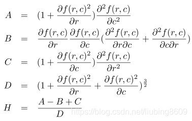
When used in context of photometric stereo, the operator derivate_vector_field offers two more parameters, which are especially designed to process the gradient field that is returned by photometric_stereo. In this case, we interpret the input vector field as gradient of the underlying surface.

In the following formulas, the input vector field is therefore noted as

where the first and second component of the input is the gradient field of the surface f(r,c). In the formulas below f_rc denotes the first derivative in column direction of the first component of the gradient field.

当在光度立体上下文中使用时，算子derivate_vector_field提供了另外两个参数，它们专门用于处理photometric_stereo返回的梯度场。在这种情况下，我们将输入向量场解释为下垫面的梯度。

在下面的公式中，输入向量场记作：

其中输入的第一个和第二个分量是曲面f(r,c)的梯度场。式中f_rc表示梯度场第一分量在列方向上的一阶导数。

'mean_curvature': Mean curvature H of the underlying surface when the input vector field VectorField is interpreted as gradient field. One application of using 'mean_curvature' is to process the vector field that is returned by photometric_stereo. After filtering the vector field, even tiny scratches or bumps can be segmented.

“mean_curvature”：当输入向量场VectorField解释为梯度场时，下垫面的平均曲率H。使用“平均曲率”的一个应用是处理photometric_stereo返回的向量场。对向量场进行滤波后，甚至可以分割出微小的划痕或凸起。

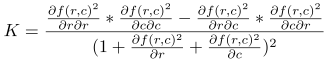
'gauss_curvature': Gaussian curvature K of the underlying surface when the input vector field VectorField is interpreted as gradient field. One application of using 'gauss_curvature' is to process the vector field that is returned by photometric_stereo. After filtering the vector field, even tiny scratches or bumps can be segmented. If the underlying surface of the vector field is developable, the Gaussian curvature is zero.

“gauss_curvature”：当输入向量场VectorField被解释为梯度场时，下垫面的高斯曲率K。使用'gauss_curvature'的一个应用程序是处理photometric_stereo返回的向量场。对向量场进行滤波后，甚至可以分割出微小的划痕或凸起。如果向量场的下表面是可展的，高斯曲率为零。

unwarp_image_vector_field

unwarp_image_vector_field — Unwarp an image using a vector field.	unwarp_image_vector_field：使用向量场反扭曲图像。
unwarp_image_vector_field(Image, VectorField : ImageUnwarped : : )	unwarp_image_vector_field(Image, VectorField : ImageUnwarped : : )
unwarp_image_vector_field unwarps the image Image using the vector field VectorField and returns the unwarped image in ImageUnwarped. The vector field must be of the semantic type 'vector_field_relative' and is typically determined with optical_flow_mg. Hence, unwarp_image_vector_field can be used to unwarp the second input image of optical_flow_mg to the first input image. It should be noted that because of the above semantics the vector field image represents an inverse transformation from the destination image of the vector field to the source image.	unwarp_image_vector_field使用向量场VectorField反扭曲图像Image，并在ImageUnwarped中返回反扭曲的图像。向量场必须是语义类型“vector_field_relative”，通常由optical_flow_mg确定。因此，unwarp_image_vector_field可用于将optical_flow_mg的第二个输入图像反扭曲到第一个输入图像。需要注意的是，由于上述语义，向量场图像表示从向量场的目标图像到源图像的逆变换。

vector_field_length

vector_field_length — Compute the length of the vectors of a vector field.	vector_field_length：计算向量场的向量长度。
vector_field_length(VectorField : Length : Mode : )	vector_field_length(VectorField : Length : Mode : )
vector_field_length compute the length of the vectors of the vector field VectorField and returns them in Length. vector_field_length only accepts vector fields of the semantic type 'vector_field_relative'. The parameter Mode can be used to specify how the lengths are computed. For Mode = 'length', the Euclidean length of the vectors is computed. For Mode = 'squared_length', the square of the length of the vectors is computed. This avoids having to compute a square root internally, which is a costly operation on many processors, and hence saves runtime on these processors. Note that the VectorField must be in relative coordinates as returned by optical_flow_mg.	vector_field_length计算向量场VectorField的长度并返回Length。vector_field_length只接受语义类型“vector_field_relative”的向量场。参数模式可用于指定如何计算长度。对于Mode = 'length'，计算向量的欧氏长度。对于Mode = 'squared_length'，计算向量长度的平方。这避免了在内部计算平方根，这在许多处理器上是一个费时的操作，因此节省了这些处理器上的运行时。注意VectorField必须在optical_flow_mg返回的相对坐标中。

HALCON：Optical Flow（光流法）

光流法基本原理

基于梯度的方法：该类方法是建立在图像亮度为常数的假设基础之上的，利用序列图像亮度的时空梯度函数来计算2D速度场（光流）。由于计算简单而且效果比较好，该方法成为使用最广泛的一种光流估计方法，此类方法的最具代表性的是Horn-Schunck光流法，它计算出的光流场是在光流基本方程的基础上引入了另外一个约束条件，即全局光流平滑约束假设。后来人们根据这种思想又提出了大量的改进算法。基于梯度的光流法在使用中存在一些问题：
第一，为了在计算光流方程时方便，一般会通过一阶泰勒级数逼近来线性化，因此当有大的运动矢量存在时会产生较大误差，从而导致估计精度降低；
第二，在进行预处理时，部分帧中噪声的存在、图像采集过程中的频谱混叠现象都将严重影响该类方法的计算精度；
第三，在有些非连续区域(比如边缘等)，图像亮度在运动方向上的平滑性约束条件会被破坏，从而会导致计算错误。
基于匹配的方法：包括基于特征和基于区域两种方法。基于特征的方法不断地对目标主要特征进行定位和跟踪，对大目标的运动和亮度变化具有鲁棒性。存在问题是光流通常很稀疏，且特征提取和精确匹配也十分困难。基于区域的方法先对类似的区域进行定位，然后通过相似区域的位移计算光流。这种方法在视频编码中得到了广泛的应用，然而它计算的光流仍不稠密。
基于频域（能量）的方法：在使用该类方法的过程中，要获得均匀流场准确的速度估计，就必须对输入图像进行时空滤波处理，即对时间和空间整合，但是这样会降低光流的时间和空间分辨率。基于频率的方法往往会涉及大量的计算，另外，要进行可靠性评价也比较困难。
基于相位的方法：由Fleet和Jepson提出的，Fleet和Jepson最先提出将相位信息用于光流计算的思想。当我们计算光流的时候，相比亮度信息，图像的相位信息更加可靠，所以利用相位信息获得的光流场具有更好的鲁棒性。基于相位的光流算法的优点是：对图像序列的适用范围较宽，而且速度估计比较精确，但也存在着一些问题：
第一，基于相位的模型有一定的合理性，但是有较高的时间复杂性；
第二，基于相位的方法通过两帧图像就可以计算出光流，但如果要提高估计精度，就需要花费一定的时间；
第三，基于相位的光流计算法对图像序列的时间混叠是比较敏感的。
神经动力学方法：利用神经网络建立的视觉运动感知的神经动力学模型，是对生物视觉系统功能与结构比较直接的模拟。