高斯模糊在图像处理中的用途及其广泛,除了常规的模糊效果外,还可用于图像金字塔分解、反走样、高低频分解、噪声压制、发光效果等等等等。正因为高斯模糊太基础,应用太广泛,所以需要尽可能深入认识这个能力,避免在实际应用中无意采坑。
一维高斯核函数
公式
G ( x ) = 1 2 π σ e − ( x − μ ) 2 2 σ 2 G(x) = \frac{1}{\sqrt{2\pi}\sigma}e^{-\frac{(x-\mu)^2}{2\sigma^2}} G(x)=2πσ1e−2σ2(x−μ)2
其中 μ \mu μ是对称轴,图像处理中通常不会考虑 μ ≠ 0 \mu \neq0 μ=0的情况,所以该参数可以忽略(本文自此向下均忽略 μ \mu μ)。
σ \sigma σ决定函数的高矮胖瘦, σ \sigma σ越小越高瘦,越大越矮胖。如果用于模糊的话,高瘦意味着中心像素对于计算结果的贡献大,而远处的像素贡献相对较小,也就是说模糊结果更多受中心像素支配,因此模糊程度就低;反之矮胖意味着模糊程度高。所以其他条件不变的情况下,增大 σ \sigma σ会加强模糊,反之会减弱模糊。
e指数前的系数保证了核函数在 ( − ∞ , + ∞ ) (-\infty, +\infty) (−∞,+∞)的积分为1,不过在图像处理中,我们显然不可能用无穷大的半径,所以会对高斯核的系数做归一化,那么e指数前的系数在归一化中就被约去了,所以干脆就不用计算。
曲线形态
下图是一维高斯核函数的曲线形态。
注意下图仍然计算了e指数前的系数,并验证了核函数的积分,表明无论 σ \sigma σ怎么变化,其积分总是为1。

# -*- coding: utf-8 -*-
import numpy as np
import matplotlib.pyplot as plt


def gaussian_1d(x, sigma):
    coef = 1. / (np.sqrt(2 * np.pi) * sigma)
    return coef * np.exp(-x * x / (2 * sigma * sigma))


def plot_gaussian_1d():
    dx = 0.01
    xx = np.arange(-10, 10, dx)
    plt.figure(0, figsize=(8, 6))
    for sigma in [0.5, 1, 2]:
        yy = gaussian_1d(xx, sigma)
        ss = np.sum(yy * dx)
        plt.plot(xx, yy, label="sigma = %0.1f, integral = %0.2f" % (sigma, ss))
    plt.legend(loc='best')
    plt.savefig('gaussian_1d.png', dpi=300)
    plt.close(0)


if __name__ == '__main__':
    plot_gaussian_1d()
有效模糊半径
一般而言,增大模糊半径会加强模糊效果。但从曲线形态可以看到,远离对称中心时,高斯核的系数将会变得非常非常小,在做图像模糊时,意味着这些远处的像素对于模糊的贡献将会变得非常小,此时增大半径几乎不会带来模糊程度的增加,但是计算量却丝毫没有减少。
所以这里应当注意一个有效模糊半径的概念。因为 σ \sigma σ会影响曲线的高矮胖瘦,所以容易知道有效模糊半径受 σ \sigma σ影响。为了定义有效模糊半径,我们必须定义一个标准,这个标准应当具有相对性概念。比如简单来说我们针对曲线某个点的数值与最大值的比来进行定义:
arg max x ( G ( x , σ ) G ( 0 , σ ) ) > l i m i t \argmax_x(\frac{G(x, \sigma)}{G(0,\sigma)}) > limit xargmax(G(0,σ)G(x,σ))>limit
如果我们把满足上式的最大x称为有效有效模糊半径,那么就可以去找一下其与 σ \sigma σ的关系了。
搞清楚有效模糊半径对于图像处理的实践很重要,避免浪费了算力却并没有得到相应的模糊效果。然而这个概念很少被讨论。

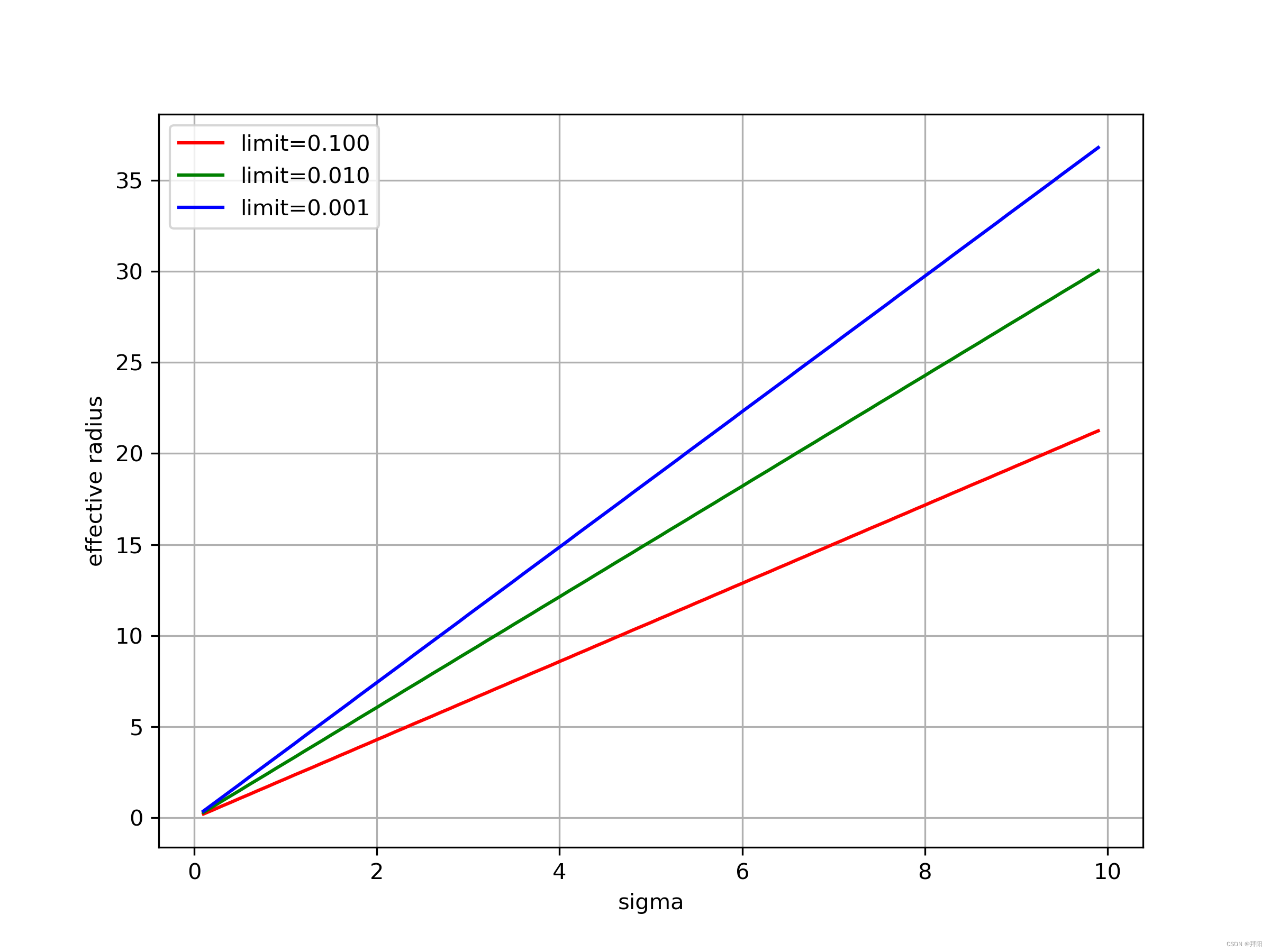
下面是不同的limit情况下sigma与有效模糊半径的关系,很容易看出来这是个线性关系。
因此,假如我们要开发一个“模糊”的功能,只开放一个模糊程度参数,那么一般而言这个参数需要跟半径挂钩,但为了让半径能真正起到作用,就需要适配的sigma,这个sigma可以使用 s i g m a = r a d i u s / a sigma = radius / a sigma=radius/a 来计算得到。针对图像模糊,根据经验,a使用[2, 2.5]之间的数字均可。
def effective_radius():
    dx = 0.01
    xx = np.arange(0, 100, dx)
    limits = [0.1, 0.01, 0.001]
    colors = ['red', 'green', 'blue']

    sigmas = np.arange(0.1, 10, 0.1)

    plt.figure(0, figsize=(8, 6))
    for i, limit in enumerate(limits):
        effective_r = []
        for sigma in sigmas:
            yy = gaussian_1d(xx, sigma)
            yy = yy / np.max(yy)
            radius = np.max(np.argwhere(yy >= limit))
            effective_r.append(radius * dx)
        plt.plot(sigmas, effective_r, color=colors[i],
                 label='limit=%0.3f' % limit)

    plt.legend(loc='best')
    plt.grid()
    plt.xlabel('sigma')
    plt.ylabel('effective radius')
    plt.savefig('effective radius', dpi=300)
    plt.close(0)
二维高斯核函数
公式
G ( x , y ) = 1 2 π σ x σ y e − ( ( x − μ x ) 2 2 σ x 2 + ( y − μ y ) 2 2 σ y 2 ) G(x,y) = \frac{1}{2\pi\sigma_x\sigma_y}e^{-(\frac{(x-\mu_x)^2 }{2\sigma_x^2} + \frac{(y-\mu_y)^2 }{2\sigma_y^2})} G(x,y)=2πσxσy1e−(2σx2(x−μx)2+2σy2(y−μy)2)
对于图像模糊来说,我们不关心平均值 μ \mu μ和前面的系数,所以公式可以简化为:
G ( x , y ) = e − ( x 2 2 σ x 2 + y 2 2 σ y 2 ) G(x,y) = e^{-(\frac{x^2 }{2\sigma_x^2} + \frac{y^2 }{2\sigma_y^2})} G(x,y)=e−(2σx2x2+2σy2y2)
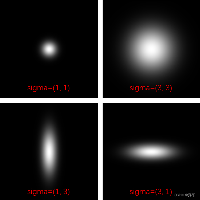
下面是生成kernel的代码和结果
# -*- coding: utf-8 -*-
import cv2
import numpy as np


def gaussian_2d(radius, sigma_x, sigma_y):
    coord = np.arange(-radius, radius, 0.01)
    xx, yy = np.meshgrid(coord, coord)
    res = np.exp(
        -(xx * xx / (sigma_x * sigma_x) + yy * yy / (sigma_y * sigma_y)) / 2)
    res = res / np.sum(res)
    return res


def plot_gaussian_2d():
    radius = 10
    sigma_x = 1.0
    sigma_y = 1.0

    kernel = gaussian_2d(radius, sigma_x, sigma_y)
    kernel = kernel / np.max(kernel)
    kernel = np.clip(np.round(kernel * 255), 0, 255)
    kernel = np.uint8(kernel)

    cv2.imwrite('radius=%d, sigma=(%d, %d).png' % (radius, sigma_x, sigma_y),
                kernel)
行列嵌套循环的高斯模糊
# -*- coding: utf-8 -*-
import cv2
import numpy as np


def gaussian_2d(radius, sigma_x, sigma_y, d_radius=1):
    coord = np.arange(-radius, radius + d_radius, d_radius)
    xx, yy = np.meshgrid(coord, coord)
    res = np.exp(-(xx * xx / (sigma_x * sigma_x) +
                   yy * yy / (sigma_y * sigma_y)) / 2)
    res = res / np.sum(res)
    return res


def convolve_2d(image, kernel, border='transparent'):
    image_height, image_width = image.shape[:2]
    kernel_height, kernel_width = kernel.shape[:2]
    radius_h = kernel_height // 2
    radius_w = kernel_width // 2

    # check: kernel_height and kernel_width must be odd
    if radius_h * 2 + 1 != kernel_height or radius_w * 2 + 1 != kernel_width:
        raise ValueError('kernel_height and kernel_width must be odd')

    res = np.zeros_like(image, dtype=np.float32)
    for row in range(image_height):
        # print(row)
        for col in range(image_width):
            pix = 0.0
            weight = 0
            for i in range(kernel_height):
                for j in range(kernel_width):
                    row_k = row + i - radius_h
                    col_k = col + j - radius_w
                    if border == 'transparent':
                        if 0 <= row_k < image_height and \
                                0 <= col_k < image_width:
                            pix += image[row_k, col_k] * kernel[i, j]
                            weight += kernel[i, j]
                    elif border == 'zero':
                        if 0 <= row_k < image_height and \
                                0 <= col_k < image_width:
                            pix += image[row_k, col_k] * kernel[i, j]
                        weight += kernel[i, j]
                    elif border == 'copy':
                        if row_k < 0:
                            row_k = 0
                        elif row_k >= image_height:
                            row_k = image_height - 1
                        if col_k < 0:
                            col_k = 0
                        elif col_k >= image_width:
                            col_k = image_width - 1
                        pix += image[row_k, col_k] * kernel[i, j]
                        weight += kernel[i, j]
                    elif border == 'reflect':
                        if row_k < 0:
                            row_k = np.abs(row_k)
                        elif row_k >= image_height:
                            row_k = 2 * (image_height - 1) - row_k
                        if col_k < 0:
                            col_k = np.abs(col_k)
                        elif col_k >= image_height:
                            col_k = 2 * (image_width - 1) - col_k
                        pix += image[row_k, col_k] * kernel[i, j]
                        weight += kernel[i, j]
                    else:
                        raise ValueError('border must be one of '
                                         '[transparent, zero, copy, reflect]')
            res[row, col] = np.float32(pix / weight)
    res = np.uint8(np.clip(np.round(res), 0, 255))
    return res


def main_gaussian_blur():
    radius = 20
    sigma_x = 10.0
    sigma_y = 10.0
    borders = ['transparent', 'zero', 'copy', 'reflect']

    image = cv2.imread('lena_std.bmp')
    kernel = gaussian_2d(radius, sigma_x, sigma_y, d_radius=1)

    for border in borders:
        blur_image = convolve_2d(image, kernel, border)
        cv2.imwrite('blur_radius=%d,sigma=(%0.1f,%0.1f),border=%s.png' % (
            radius, sigma_x, sigma_y, border), blur_image)
上面代码仅用于示例计算流程,因为python的for循环特别慢,所以只要kernel稍微大那么一些,上面的代码就要运行非常非常久。由于图像需要在两个方向循环,kernel也需要在两个方向循环,所以整个下来计算量是o(n^4),特别慢。
除了常规的图像高斯模糊外,上面代码还示例了几种边界条件:
- transparent:超出边界的索引不参与计算,此种边界条件必需累加weight,最后用累加得到的weight做归一化。这种边界条件因为必须要对weight做累加,所以计算量略大一些些,但效果是几种边界条件中最好最稳定的。
- zero:超出边界的索引用0代替。因为0代表黑色,随着kernel增大,越来越多的0参与到了边界的模糊中,所以这种边界条件会引起黑边,效果最差。但是对于并行加速来讲,其实现是比较容易的。在神经网络的卷积中使用非常多,但是传统图像处理中尽量避免用这种边界条件。
- copy:超出边界的索引使用最近的边缘像素值,效果中规中矩,实现也简单。
- reflect:超出边界的索引,以边界为对称中心取图像内部对应位置的像素值,索引的计算会有些麻烦,特别是当kernel尺寸非常大时,以至于镜像的索引超过了对面的边界。但是当kernel尺寸不那么极端时,这种边界条件的效果一般还不错。
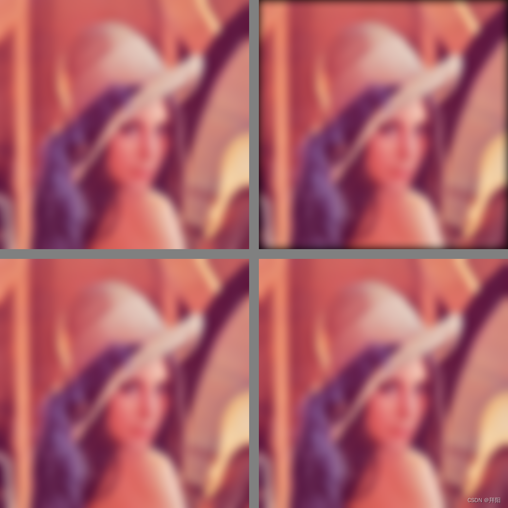
下图是4中边界条件的效果,radius=20,sigma=10。
左上:transparent,右上:zero
左下:copy, 右下:reflect
行列分离的高斯模糊
高斯模糊使用嵌套循环显然是很差劲的写法。在实践中,一般我们会写成行列分离的形式,此时计算量从o(n^4) 降低到 o(n^3)。
上面我们写过二维高斯核函数为:
G ( x , y ) = e − ( x 2 2 σ x 2 + y 2 2 σ y 2 ) G(x,y) = e^{-(\frac{x^2 }{2\sigma_x^2} + \frac{y^2 }{2\sigma_y^2})} G(x,y)=e−(2σx2x2+2σy2y2)
注意此函数可以拆开写成x,y分离的形式。
记
G ( x ) = e − x 2 2 σ x 2 G ( y ) = e − y 2 2 σ y 2 G(x) = e^{-\frac{x^2 }{2\sigma_x^2}} \\[2ex] G(y) = e^{-\frac{y^2 }{2\sigma_y^2}} G(x)=e−2σx2x2G(y)=e−2σy2y2
那么有:
G ( x , y ) = e − x 2 2 σ x 2 ⋅ e − y 2 2 σ y 2 = G ( x ) G ( y ) G(x,y) = e^{-\frac{x^2 }{2\sigma_x^2}} \cdot e^{-\frac{y^2 }{2\sigma_y^2}}=G(x)G(y) G(x,y)=e−2σx2x2⋅e−2σy2y2=G(x)G(y)
然后一个高斯模糊的计算过程为:
b l u r ( x , y ) = ∫ ∫ I ( x , y ) G ( x , y ) d x d y = ∫ ∫ I ( x , y ) G ( x ) G ( y ) d x d y = ∫ [ ∫ I ( x , y ) G ( x ) d x ] ⋅ G ( y ) d y ( 写成离散形式 ) = ∑ y i [ ∑ x i I ( x i , y i ) G ( x i ) ] G ( y i ) \begin{aligned} blur(x,y) &= \int \int I(x,y)G(x,y)dxdy \\[2ex] &= \int \int I(x,y)G(x)G(y)dxdy \\[2ex] &=\int [\int I(x,y)G(x)dx] \cdot G(y)dy \\[2ex] & (写成离散形式) \\[2ex] & =\sum_{y_i} [\sum_{x_i} I(x_i,y_i)G(x_i)]G(y_i) \end{aligned} blur(x,y)=∫∫I(x,y)G(x,y)dxdy=∫∫I(x,y)G(x)G(y)dxdy=∫[∫I(x,y)G(x)dx]⋅G(y)dy(写成离散形式)=yi∑[xi∑I(xi,yi)G(xi)]G(yi)
也就是说在x方向进行模糊,然后对这个中间结果在y方向再做模糊即可,每次只在一个方向做循环,并且这两个循环不是嵌套,而是分离的。下面代码没有再实现多种边界条件,只写了transparent类型的。
# -*- coding: utf-8 -*-
import cv2
import numpy as np


def gaussian_1d(radius, sigma, d_radius=1):
    xx = np.arange(-radius, radius + d_radius, d_radius)
    res = np.exp(-xx * xx / (sigma * sigma) / 2)
    res = res / np.sum(res)
    return res


def convolve_2d_xy(image, kernel_x, kernel_y):
    image_height, image_width = image.shape[:2]
    kernel_x_len = len(kernel_x)
    kernel_y_len = len(kernel_y)
    radius_x = kernel_x_len // 2
    radius_y = kernel_y_len // 2

    # check: kernel_height and kernel_width must be odd
    if radius_x * 2 + 1 != kernel_x_len or radius_y * 2 + 1 != kernel_y_len:
        raise ValueError('kernel size must be odd')

    res = np.zeros_like(image, dtype=np.float32)
    # convolve in x direction
    for row in range(image_height):
        for col in range(image_width):
            pix = 0.0
            weight = 0
            for j in range(kernel_x_len):
                col_k = col + j - radius_x
                if 0 <= col_k < image_width:
                    pix += image[row, col_k] * kernel_x[j]
                    weight += kernel_x[j]
            res[row, col] = pix / weight

    # convolve in y direction
    image = res.copy()
    for col in range(image_width):
        for row in range(image_height):
            pix = 0.0
            weight = 0
            for i in range(kernel_y_len):
                row_k = row + i - radius_y
                if 0 <= row_k < image_height:
                    pix += image[row_k, col] * kernel_y[i]
                    weight += kernel_y[i]
            res[row, col] = pix / weight
    res = np.uint8(np.clip(np.round(res), 0, 255))
    return res


def main_gaussian_blur_xy():
    radius = 20
    sigma_x = 10.0
    sigma_y = 10.0

    image = cv2.imread('lena_std.bmp')
    kernel_x = gaussian_1d(radius, sigma_x, d_radius=1)
    kernel_y = gaussian_1d(radius, sigma_y, d_radius=1)

    blur_image = convolve_2d_xy(image, kernel_x, kernel_y)
    cv2.imwrite('xy_blur_radius=%d,sigma=(%0.1f,%0.1f).png' % (
        radius, sigma_x, sigma_y), blur_image)
行列分离的耗时在我电脑上大概是45s,嵌套循环大概需要1020秒。尽管python的循环特别慢,这个时间对比可能做不得数,但是量级上的差异还是比较能说明问题了。
下面左图是之前嵌套循环得到的结果,中间是行列分离得到的结果,右图是两者的差的绝对值再乘以50,结果来看两个模糊的结果完全一样。

加上step的高斯模糊
当模糊的radius非常大时候,可以适当加上一些step来节省计算。
此时应当注意,为了达到预想中的模糊效果,不仅image patch与kernel乘加时的索引需要加上step,kernel系数的计算也需要加上step,不然与不加step时候的系数会有很大差异。
# -*- coding: utf-8 -*-
import cv2
import numpy as np
import time
def gaussian_1d(radius, sigma, d_radius=1.0):
xx = np.arange(-radius, radius + d_radius, d_radius)
res = np.exp(-xx * xx / (sigma * sigma) / 2)
res = res / np.sum(res)
return res
def convolve_2d_xy_step(image, kernel_x, kernel_y, step):
image_height, image_width = image.shape[:2]
kernel_x_len = len(kernel_x)
kernel_y_len = len(kernel_y)
radius_x = kernel_x_len // 2
radius_y = kernel_y_len // 2
# check: kernel_height and kernel_width must be odd
if radius_x * 2 + 1 != kernel_x_len or radius_y * 2 + 1 != kernel_y_len:
raise ValueError('kernel size must be odd')
res = np.zeros_like(image, dtype=np.float32)
# convolve in x direction
for row in range(image_height):
for col in range(image_width):
pix = 0.0
weight = 0
for j in range(kernel_x_len):
col_k = int(round(col + (j - radius_x) * step))
if 0 <= col_k < image_width:
pix += image[row, col_k] * kernel_x[j]
weight += kernel_x[j]
res[row, col] = pix / weight
# convolve in y direction
image = res.copy()
for col in range(image_width):
for row in range(image_height):
pix = 0.0
weight = 0
for i in range(kernel_y_len):
row_k = int(round(row + (i - radius_y) * step))
if 0 <= row_k < image_height:
pix += image[row_k, col] * kernel_y[i]
weight += kernel_y[i]
res[row, col] = pix / weight
res = np.uint8(np.clip(np.round(res), 0, 255))
return res
def main_gaussian_blur_xy():
radius = 20
sigma_x = 10.0
sigma_y = 10.0
step = 4.0
image = cv2.imread('lena_std.bmp')
kernel_x = gaussian_1d(radius, sigma_x, d_radius=step)
kernel_y = gaussian_1d(radius, sigma_y, d_radius=step)
blur_image = convolve_2d_xy_step(image, kernel_x, kernel_y, step)
cv2.imwrite('xy_blur_radius=%d,sigma=(%0.1f,%0.1f)_step.png' % (
radius, sigma_x, sigma_y), blur_image)
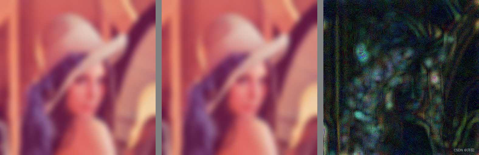
下面左图是之前嵌套循环得到的结果,中间是行列分离+step=4得到的结果,右图是两者的差的绝对值再乘以50。
此时计算出来的diff已经不再是全零,如果仔细看中间的结果,显示出了一些块状纹理,表明模糊的品质已经开始受到影响。
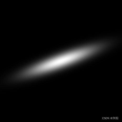
任意二维高斯核的生成
这里任意高斯核指的是任意长宽比,且存在旋转角度的高斯核。
公式推导的思路是,把高斯核G(x,y)看做是一个图像,然后用图像旋转的思路来改造二维高斯核的公式。
下面我们再次把高斯核公式摆在这里。
G ( x , y ) = e − ( x 2 2 σ x 2 + y 2 2 σ y 2 ) G(x,y) = e^{-(\frac{x^2 }{2\sigma_x^2} + \frac{y^2 }{2\sigma_y^2})} G(x,y)=e−(2σx2x2+2σy2y2)
根据图像旋转的原理,当图像中某个点(x, y)以圆心作为旋转中心,沿逆时针旋转后,新的点(x’, y’)的坐标公式为:
{ x ′ = x ∗ c o s θ − y ∗ s i n θ y ′ = x ∗ s i n θ + y ∗ c o s θ \begin{cases} x' = x*cos\theta - y*sin\theta \\ y' = x*sin\theta + y*cos\theta \end{cases} \\[4ex] {
x′=x∗cosθ−y∗sinθy′=x∗sinθ+y∗cosθ
将其代入高斯核公式,并且方便起见仍以(x, y)来表示,那么有:
G ( x , y ) = e − ( ( x ∗ c o s θ − y ∗ s i n θ ) 2 2 σ x 2 + ( x ∗ s i n θ + y ∗ c o s θ ) 2 2 σ y 2 ) = e − ( x 2 ∗ c o s 2 θ + y 2 ∗ s i n 2 θ − 2 x y ∗ s i n θ c o s θ 2 σ x 2 + x 2 s i n 2 θ + y 2 ∗ c o s 2 θ + 2 x y ∗ s i n θ c o s θ 2 σ y 2 ) = e − ( x 2 ( c o s 2 θ 2 σ x 2 + s i n 2 θ 2 σ y 2 ) + x y ( − s i n 2 θ 2 σ x 2 + s i n 2 θ 2 σ y 2 ) + y 2 ( s i n 2 θ 2 σ x 2 + c o s 2 θ 2 σ y 2 ) ) \begin{aligned} G(x,y) &= e^{-(\frac{(x*cos\theta - y*sin\theta)^2 }{2\sigma_x^2} + \frac{(x*sin\theta + y*cos\theta)^2 }{2\sigma_y^2})} \\[2ex] &=e^{-(\frac{x^2*cos^2\theta + y^2*sin^2\theta -2xy*sin\theta cos\theta}{2\sigma_x^2} + \frac{x^2sin^2\theta + y^2*cos^2\theta + 2xy*sin\theta cos\theta }{2\sigma_y^2})} \\[2ex] &=e^{-(x^2(\frac{cos^2\theta}{2\sigma_x^2} + \frac{sin^2\theta}{2\sigma_y^2}) + xy(-\frac{sin2\theta}{2\sigma_x^2} + \frac{sin2\theta}{2\sigma_y^2}) + y^2( \frac{sin^2\theta}{2\sigma_x^2} + \frac{cos^2\theta}{2\sigma_y^2} ))} \end{aligned} G(x,y)=e−(2σx2(x∗cosθ−y∗sinθ)2+2σy2(x∗sinθ+y∗cosθ)2)=e−(2σx2x2∗cos2θ+y2∗sin2θ−2xy∗sinθcosθ+2σy2x2sin2θ+y2∗cos2θ+2xy∗sinθcosθ)=e−(x2(2σx2cos2θ+2σy2sin2θ)+xy(−2σx2sin2θ+2σy2sin2θ)+y2(2σx2sin2θ+2σy2cos2θ))
上述公式就是任意二维高斯核的样子。
下面是python的实现代码和图,将一个沿横向比较长的kernel逆时针旋转了20度。
# -*- coding: utf-8 -*-
import cv2
import numpy as np


def generalized_gaussian_kernel(ksize,
                                sigma_x,
                                sigma_y=None,
                                angle=0.0):
    """
    Generate generalized gaussian kernel.

    Parameters
    ----------
    ksize: kernel size, one integer or a list/tuple of two integers, must be
        odd
    sigma_x: standard deviation in x direction
    sigma_y: standard deviation in y direction
    angle: rotate angle, anti-clockwise

    Returns
    -------
    kernel: generalized gaussian blur kernel
    """
    # check parameters
    if not isinstance(ksize, (tuple, list)):
        ksize = [ksize, ksize]
    else:
        ksize = list(ksize)
    ksize[0] = ksize[0] // 2 * 2 + 1
    ksize[1] = ksize[1] // 2 * 2 + 1

    if sigma_y is None:
        sigma_y = sigma_x

    # meshgrid coordinates
    radius_x = ksize[0] // 2
    radius_y = ksize[1] // 2
    x = np.arange(-radius_x, radius_x + 1, 1)
    y = np.arange(-radius_y, radius_y + 1, 1)
    xx, yy = np.meshgrid(x, y)

    # coefficients of coordinates
    angle = angle / 180 * np.pi
    cos_square = np.cos(angle) ** 2
    sin_square = np.sin(angle) ** 2
    sin_2 = np.sin(2 * angle)

    alpha = 0.5 / (sigma_x * sigma_x)
    beta = 0.5 / (sigma_y * sigma_y)
    a = cos_square * alpha + sin_square * beta
    b = -sin_2 * alpha + sin_2 * beta
    c = sin_square * alpha + cos_square * beta

    # generate and normalize kernel
    kernel = np.exp(-(a * xx * xx + b * xx * yy + c * yy * yy))
    kernel = kernel / np.sum(kernel)
    return kernel


if __name__ == '__main__':
    ksize = (511, 511)
    sigma_x = 100.0
    sigma_y = 20.0
    angle = 20.0

    gaussian_kernel = generalized_gaussian_kernel(ksize=ksize,
                                                  sigma_x=sigma_x,
                                                  sigma_y=sigma_y,
                                                  angle=angle)
    gaussian_kernel = gaussian_kernel / np.max(gaussian_kernel)
    gaussian_kernel = np.uint8(np.round(gaussian_kernel * 255))
    cv2.imwrite('generalized_gaussian_kernel_1.png', gaussian_kernel)