引言
霍夫变换(Hough Transform)换于1962年由Paul Hough 首次提出,后于1972年由Richard Duda和Peter Hart推广使用,是图像处理中从图像中检测几何形状的基本方法之一。经典霍夫变换用来检测图像中的直线,后来霍夫变换经过扩展可以进行任意形状物体的识别,例如圆和椭圆。
霍夫变换运用两个坐标空间之间的变换将在一个空间中具有相同形状的曲线或直线映射到另一个坐标空间的一个点上形成峰值,从而把检测任意形状的问题转化为统计峰值问题。
霍夫变换检测直线原理
在笛卡尔坐标系下两点确定的直线为 y = kx+q,考虑已知的A,B两点,则可以确定唯一的 k,q

若以k, q为自变量、因变量可以绘制 霍夫坐标系,那么笛卡尔坐标系下的直线则对应霍夫坐标系下的一个点:

相反,考虑在笛卡尔坐标系下的一个点(x1, y1) ,过这一点的直线方程为:q = -x1k+y1
此时该方程表示霍夫空间下的一条直线:

如果有三个共线的点,则可以看到笛卡尔坐标下共线的点在霍夫空间交于一点,因为笛卡尔坐标系下的直线对应霍夫空间中的一个点。

因为原始图像直角坐标空间中的特殊直线x=c(垂直x轴,直线的斜率为无穷大)是没办法在基于直角坐标系的参数空间中表示的。所以在实际应用中,霍夫空间采用极坐标系进行表示。

在极坐标下,霍夫空间的直线将会变成曲线。在笛卡尔坐标系中,直线由无数个点组成,对应到霍夫空间就是无数条直线或曲线相交于一点,因此在霍夫空间中通过寻找极大值可以确定直线的参数。

如前所述,霍夫直线检测就是把图像空间中的直线变换到参数空间中的点,通过统计特性来解决检测问题。具体来说,如果一幅图像中的像素构成一条直线,那么这些像素坐标值(x, y)在参数空间对应的曲线一定相交于一个点,所以我们只需要将图像中的所有像素点(坐标值)变换成参数空间的曲线,并在参数空间检测曲线交点就可以确定直线了。
在理论上,一个点对应无数条直线或者说任意方向的直线,但在实际应用中,我们必须限定直线的数量(即有限数量的方向)才能够进行计算。
因此,我们将直线的方向θ离散化为有限个等间距的离散值,参数ρ也就对应离散化为有限个值,于是参数空间不再是连续的,而是被离散量化为一个个等大小网格单元。将图像空间(直角坐标系)中每个像素点坐标值变换到参数空间(极坐标系)后,所得值会落在某个网格内,使该网格单元的累加计数器加1。当图像空间中所有的像素都经过霍夫变换后,对网格单元进行检查,累加计数值最大的网格,其坐标值(ρ0, θ0)就对应图像空间中所求的直线。

以上就是霍夫直线检测算法要做的,它检测图像中每个像素点在参数空间对应曲线之间的交点,如果交于一点的曲线的数量超过了阈值,那就可以认为这个交点(ρ,θ)在图像空间中对应一条直线。
基于opencv实现
使用opencv的霍夫变换检测直线函数HoughLines、HoughLinesP,相关的函数说明如下:
cv2.HoughLines(
	image, 				# 原图像。
	rho, 				# 累加器的距离分辨率(以像素为单位)。
	theta, 				# 累加器的弧度角分辨率。
	threshold[, 		# 累加器阈值参数。只返回那些获得足够投票的直线(> threshold)。
	lines[, 			# 返回的线,格式为 [[rho_1,theta_1], [rho_2,theta_2], ...]
	srn[, 				# 对于多尺度 Hough 变换,它是距离分辨率 ρ 的一个除数。
						  粗的累加器距离分辨率为 ρ,精确的累加器分辨率为 ρ/srn。
						  如果同时使用 srn = 0 和 stn = 0,则使用经典的 Hough 变换。
						  否则,这两个参数都应该是正数。
	stn[, 				# 对于多尺度 Hough 变换,它是距离分辨率 θ 的除数。
	min_theta[,			# 对于标准和多尺度霍夫变换,最小角度检查线。必须在0和max_theta之间。
    max_theta			# 对于标准和多尺度霍夫变换,检查线路的最大角度。必须在 min_theta 和 cv2.CV_pi 之间。
    ]]]]]) -> lines
cv2.HoughLinesP(
	image, 				# 源图像。
	rho, 				# 累加器的距离分辨率(以像素为单位)。
	theta, 				# 累加器的弧度角分辨率。
	threshold[, 		# 累加器阈值参数。只返回那些获得足够投票的直线(> threshold)。
	lines[, 			# 返回线结果,格式为 [[xmin, ymin, xmax, ymax], ...]。
	minLineLength[, 	# 最短线段长度。
	maxLineGap]]]		# 点连接成线的最大距离。
	) -> lines
代码实现如下:
edge = cv2.Canny(np.array(img, dtype='uint8'), 1743, 3400, apertureSize=7, L2gradient=True)
plt.imshow(edge)
plt.show()
# ============================使用opencv霍夫变换=============================
lines = cv2.HoughLines(edge, rho=1, theta=np.pi/180, threshold=round(800*scale_factor))
if lines is not None:
    for line in lines:
        rho, theta = line[0]
        a = np.cos(theta)
        b = np.sin(theta)
        x0 = a * rho
        y0 = b * rho
        x1 = int(x0 + 1000 * (-b))
        y1 = int(y0 + 1000 * (a))
        x2 = int(x0 - 1000 * (-b))
        y2 = int(y0 - 1000 * (a))
        cv2.line(img, (x1, y1), (x2, y2), (250, 20, 250), 2)

cv2.imshow("img", img)
cv2.imshow("edge", edge)
cv2.waitKey(0)
cv2.destroyAllWindows()
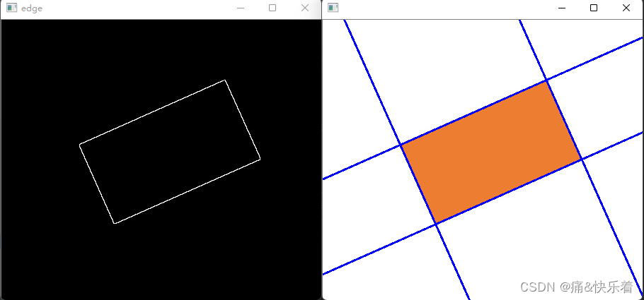
效果如下:
其中可以看到对于上述实例OpenCV自带的函数能够很好的对直线进行检测,但是,当图像比较复杂时需要对阈值进行控制,否则将会得到很多不符合预期的结果。
基于霍夫变换检测ROI原理
由上述可知,通过霍夫变换检测直线可以对目标图像的矩形ROI进行检测,然而使用OpenCV自带的霍夫变换检测直线函数并不是很方便。我们知道:
- 在霍夫域中长直线导致高水平的斑点
- 平行线具有相同的角度,因此它们对应的点在霍夫域上出现在相同的θ值上。
- 垂直线之间的距离为θ=π /2
- 由于准直线是两对几乎平行和垂直的,因此在Hough域分析中寻找两对θ值几乎相同的亮点,它们之间的距离约为θ=π /2。
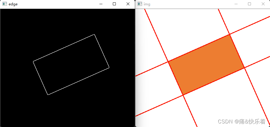
- 据此我们可以得到矩形ROI的四条直线,也即是实现了矩形ROI的检测。

基于python实现霍夫变换检测矩形ROI
算法步骤:
(1)初始化累加器 H全零;
(2)遍历图像中的每一个边缘点;
(3)找到 H中局部最大值的点以及相隔π/2的点;
(4)将点 (θ,ρ)转换为图像中的直线。
# 测试,笛卡尔坐标系到霍夫域的转换
rho = []
rad = []
for theta in range(max_theta):
    # print(theta)
    theta = np.pi*theta/180
    rad.append(theta)
    rho1 = 100 * np.cos(theta) + 100 * np.sin(theta)
    rho.append(rho1)
plt.plot([0, x_data[-1]], [0, 0])
plt.plot(x_data, rho), plt.xlabel('theta'), plt.ylabel('rho')
plt.xlim([0, 180])
plt.show()

将笛卡尔坐标系(图像坐标)转换到霍夫域(参数坐标)。
H = np.zeros([round(edge.shape[0]*3.2), max_theta])
points = []  # 边缘点集
for y in range(edge.shape[0]):
    for x in range(edge.shape[1]):
        if edge[y, x] > 0:
            p1 = [x, y]
            points.append(p1)

for p2 in points:
    # print(p2)
    for theta in range(max_theta):
        theta_rad = np.pi * theta / 180
        rho = p2[0] * np.cos(theta_rad) + p2[1] * np.sin(theta_rad)
        H[round(rho+H.shape[0]/2), round(theta)] += 1  # x,y,height的中点为坐标原点
# H[:, 0] = H[:, 0] + H[:, -1]

H = np.flipud(H)

hough_max = np.max(H, 0)
# plt.subplot(211), plt.imshow(H)
# plt.subplot(212), plt.plot(x_data, hough_max)
plt.imshow(H)
plt.show()

在霍夫域寻找平行和垂直线,总计四个点,并将其在霍夫图像中进行显示。
# 在霍夫域寻找平行和垂直线,四个点
theta_rho_max1 = np.argmax(hough_max)
theta_rho_max2 = theta_rho_max1 + 90
theta_rho_max2 = theta_rho_max2 % 180
print(theta_rho_max1)
print(theta_rho_max2)
rho_max1 = round(hough_max0[theta_rho_max1])  # 得到theta最大值的第一个rho
temp = np.where(H[:, theta_rho_max1] == rho_max1)
rho_max1_index = temp[0][0]
rho_max11_index = round(hough_max2(H[:, theta_rho_max1], rho_max1_index))
rho_max2 = round(hough_max0[theta_rho_max2])
temp = np.where(H[:, theta_rho_max2] == rho_max2)
rho_max2_index = temp[0][0]
rho_max22_index = round(hough_max2(H[:, theta_rho_max2], rho_max2_index))

# 在霍夫图像中标记处检测到的四个点
H[rho_max1_index, theta_rho_max1] = 100
H[rho_max11_index, theta_rho_max1] = 100
H[rho_max2_index, theta_rho_max2] = 100
H[rho_max22_index, theta_rho_max2] = 100
plt.imshow(H), plt.xlim([0, 180])
plt.show()

完整代码如下:
# -*- coding: UTF-8 -*-
"""
霍夫变换实现并将其用于检测ROI
"""
import numpy as np
import matplotlib.pyplot as plt
import cv2

img = cv2.imread('../images/hough_test2.jpg', -1)
scale_factor = 1.0/2.0
img = cv2.resize(img, None, fx=scale_factor, fy=scale_factor)
gray = cv2.cvtColor(img, cv2.COLOR_BGR2GRAY)
print(np.shape(gray))

# ret, bw = cv2.threshold(gray, 0, 255, cv2.THRESH_OTSU)
edge = cv2.Canny(gray, 17430*scale_factor, 34000*scale_factor, apertureSize=7, L2gradient=True)

# cv2.imshow("", bw)
# cv2.waitKey()
# edge = cv2.Canny(gray, 17, 34, apertureSize=7, L2gradient=True)
# ============================使用opencv霍夫变换=============================
# lines = cv2.HoughLines(edge, rho=1, theta=np.pi/180, threshold=round(170*scale_factor))
# if lines is not None:
#     for line in lines:
#         rho, theta = line[0]
#         a = np.cos(theta)
#         b = np.sin(theta)
#         x0 = a * rho
#         y0 = b * rho
#         x1 = int(x0 + 1000 * (-b))
#         y1 = int(y0 + 1000 * (a))
#         x2 = int(x0 - 1000 * (-b))
#         y2 = int(y0 - 1000 * (a))
#         cv2.line(img, (x1, y1), (x2, y2), (0, 20, 250), 2)
# cv2.imshow("img", img)
# cv2.imshow("edge", edge)
# cv2.waitKey()
# cv2.destroyAllWindows()
# ============================自己实现霍夫变换=============================


def mean_filter1(data, fsize):
    l = np.shape(data)[0]
    dst = np.zeros([l, 1])
    hsize = round(fsize / 2)
    for i in range(l):
        left = i - hsize
        right = i + hsize
        if left < 0:
            left = 0
        if right > l-1:
            right = l-1
        dst[i] = np.mean(data[left:right], 0)
    return dst


def hough_max2(arr, m1=0):
    l = len(arr)
    m = 0
    max_index = 0
    for i in range(l):
        if arr[i] > m and i != m1:
            m = arr[i]
            max_index = i
    return max_index


max_theta = 181
x_data = np.arange(max_theta)

# 测试
rho = []
rad = []
for theta in range(max_theta):
    # print(theta)
    theta = np.pi*theta/180
    rad.append(theta)
    rho1 = 100 * np.cos(theta) + 100 * np.sin(theta)
    rho.append(rho1)
plt.plot([0, x_data[-1]], [0, 0])
plt.plot(x_data, rho), plt.xlabel('theta'), plt.ylabel('rho')
plt.xlim([0, 180])
plt.show()

H = np.zeros([round(edge.shape[0]*3.2), max_theta])
points = []  # 边缘点集
for y in range(edge.shape[0]):
    for x in range(edge.shape[1]):
        if edge[y, x] > 0:
            p1 = [x, y]
            points.append(p1)


for p2 in points:
    # print(p2)
    for theta in range(max_theta):
        theta_rad = np.pi * theta / 180
        rho = p2[0] * np.cos(theta_rad) + p2[1] * np.sin(theta_rad)
        H[round(rho+H.shape[0]/2), round(theta)] += 1  # x,y,height的中点为坐标原点
# H[:, 0] = H[:, 0] + H[:, -1]

H = np.flipud(H)

hough_max = np.max(H, 0)
# plt.subplot(211), plt.imshow(H)
# plt.subplot(212), plt.plot(x_data, hough_max)
plt.imshow(H)
plt.show()

hough_max0 = hough_max
hough_max = mean_filter1(hough_max, 10)
kernelSize = 10
hough_max_nms = np.zeros([hough_max.shape[0]])
for i in range(hough_max.shape[0]):
    temp = hough_max[i:i+kernelSize]
    max1 = np.max(temp)
    hough_max_nms[i] = max1

for i in range(hough_max.shape[0]):
    if hough_max[i] == hough_max_nms[i]:
        hough_max_nms[i] = hough_max[i]
    else:
        hough_max_nms[i] = 0

plt.plot(x_data, hough_max)
for i in range(hough_max_nms.shape[0]):
    if hough_max_nms[i] > 0:
        plt.scatter(x_data[i], hough_max_nms[i], c='r')
plt.xlabel('theta'), plt.ylabel('rho')
plt.show()

# 在霍夫域寻找平行和垂直线,四个点
theta_rho_max1 = np.argmax(hough_max)
theta_rho_max2 = theta_rho_max1 + 90
theta_rho_max2 = theta_rho_max2 % 180
print(theta_rho_max1)
print(theta_rho_max2)
rho_max1 = round(hough_max0[theta_rho_max1])  # 得到theta最大值的第一个rho
temp = np.where(H[:, theta_rho_max1] == rho_max1)
rho_max1_index = temp[0][0]
rho_max11_index = round(hough_max2(H[:, theta_rho_max1], rho_max1_index))
rho_max2 = round(hough_max0[theta_rho_max2])
temp = np.where(H[:, theta_rho_max2] == rho_max2)
rho_max2_index = temp[0][0]
rho_max22_index = round(hough_max2(H[:, theta_rho_max2], rho_max2_index))

# 在霍夫图像中标记处检测到的四个点
H[rho_max1_index, theta_rho_max1] = 100
H[rho_max11_index, theta_rho_max1] = 100
H[rho_max2_index, theta_rho_max2] = 100
H[rho_max22_index, theta_rho_max2] = 100
plt.imshow(H), plt.xlim([0, 180])
plt.show()

hp1 = [rho_max1_index, theta_rho_max1]
hp2 = [rho_max11_index, theta_rho_max1]
hp3 = [rho_max2_index, theta_rho_max2]
hp4 = [rho_max22_index, theta_rho_max2]
hough_points = [hp1, hp2, hp3, hp4]
print(hough_points)

for line in hough_points:
    rho = -(line[0] - H.shape[0]/2 + 1)
    theta = line[1]
    theta = np.pi * theta / 180
    a = np.cos(theta)
    b = np.sin(theta)
    x0 = a*rho  # 转换为笛卡尔坐标
    y0 = b*rho
    x1 = int(x0 + 1000*(-b))
    y1 = int(y0 + 1000*(a))
    x2 = int(x0 - 1000*(-b))
    y2 = int(y0 - 1000*(a))

    cv2.line(img, (x1, y1), (x2, y2), (250, 0, 0), 2)
cv2.imshow("edge", edge)
cv2.imshow("", img)
cv2.waitKey()
cv2.destroyAllWindows()