Gempy 是一个开源 Python 库,用于生成完整的 3D 结构地质模型。 该库是一个完整的开发,用于从界面、断层和层方向创建地质模型,它还关联地质层的顺序以表示岩石侵入和断层顺序。

推荐:用 NSDT设计器 快速搭建可编程3D场景。
地质建模算法基于通用协同克里格插值,并支持 Numpy、PyMC3 和 Theano 等高端 Python 数学库。
Gempy 创建一个网格模型,可以使用 Matplotlib 将其可视化为 2D 剖面,或者将 3D 几何对象可视化为 VTK 对象,从而允许在 Paraview 上表示地质模型,以进行自定义切片、过滤、透明度和样式设置。
本教程提供具有 5 层和 1 个断层的分层地质设置的基本示例。 为了使大多数用户能够完全访问本教程,我们创建了一个关于如何使用 Anaconda 存储库发行版在 Windows 上安装 Gempy 的补充教程。
可以从此链接下载本教程的输入文件。
1、设置Python环境
在这一部分中,我们导入本教程所需的库。 该脚本需要 Gempy 以及 Numpy 和 Matplotlib。 我们在脚本单元格之后配置 Jupyter 选项以交互式表示 Matplotlib 图形(%matplotlib inline)。
请注意,警告只是用户在运行脚本时必须记住的消息,并不意味着代码失败。 由于本教程是在 Windows 上进行的,因此一些补充库无法安装,但地质建模代码的整体性能是完整的。
# Embedding matplotlib figures in the notebooks
%matplotlib inline

# Importing GemPy
import gempy as gp

# Importing auxiliary libraries
import numpy as np
import matplotlib.pyplot as plt
2、地质模型对象的创建和地理学定义
本教程在 2 公里 x 2 公里 x 2 公里的延伸范围内创建一个 100 列 x 100 行 x 100 层的网格。 更高的分辨率是可能的,但计算时间会更长。 坐标系为局部坐标系,后续教程将使用UTM坐标来评估Gempy的性能。
方向和地质接触面从 CSV 文件导入并转换为 Pandas 数据框。 然后定义地质系列(断层/地层)以及地质地层序列。
值得一提的是,故障必须独立插入,其中最年轻的是第一个条目。
# Importing the data from CSV-files and setting extent and resolution
geo_data = gp.create_data([0,2000,0,2000,0,2000],[100,100,100],
                          path_o = "../Txt/simple_fault_model_orientations.csv", # importing orientation (foliation) data
                          path_i = "../Txt/simple_fault_model_points.csv") # importing point-positional interface data
gp.get_data(geo_data).loc[:,['X','Y','Z','formation']].head()
X	Y	Z	formation
interfaces	52	700.0	1000.0	900.0	Main_Fault
53	600.0	1000.0	600.0	Main_Fault
54	500.0	1000.0	300.0	Main_Fault
55	800.0	1000.0	1200.0	Main_Fault
56	900.0	1000.0	1500.0	Main_Fault
# Assigning series to formations as well as their order (timewise)
gp.set_series(geo_data, {"Fault_Series":'Main_Fault',
                      "Strat_Series": ('Sandstone_2','Siltstone', 'Shale', 'Sandstone_1')},
                       order_series = ["Fault_Series", 'Strat_Series'],
                       order_formations=['Main_Fault',
                                         'Sandstone_2','Siltstone', 'Shale', 'Sandstone_1',
                                         ], verbose=0)
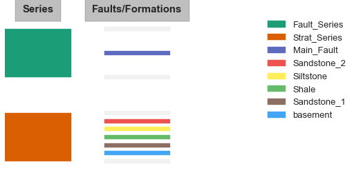
3、地质层序图
Gempy 具有一些有用的特征来表示定义的地质系列和地层序列。
gp.get_sequential_pile(geo_data)
<gempy.plotting.sequential_pile.StratigraphicPile at 0x107149e8>
4、输入数据的审核
可以通过 Gempy 的“.get_”函数访问用于地质模型构建的不同数据集。
# Review of the centroid coordinates from the model grid
gp.get_grid(geo_data).values

array([[   10.,    10.,    10.],
       [   10.,    10.,    30.],
       [   10.,    10.,    50.],
       ...,
       [ 1990.,  1990.,  1950.],
       [ 1990.,  1990.,  1970.],
       [ 1990.,  1990.,  1990.]], dtype=float32)

# Defined interfases from the input CSV data
gp.get_data(geo_data, 'interfaces').loc[:,['X','Y','Z','formation']].head()
X	Y	Z	formation
52	700.0	1000.0	900.0	Main_Fault
53	600.0	1000.0	600.0	Main_Fault
54	500.0	1000.0	300.0	Main_Fault
55	800.0	1000.0	1200.0	Main_Fault
56	900.0	1000.0	1500.0	Main_Fault
# Defined layer orientations from the input CSV data
gp.get_data(geo_data, 'orientations').loc[:,['X','Y','Z','formation','azimuth']]
| X | Y | Z | formation | azimuth |
|---|---|---|---|---|
| 2 | 500 | 1000 | 864.602 | Main_Fault |
| 1 | 400 | 1000 | 1400.000 | Sandstone_2 |
| 0 | 1000 | 1000 | 950.000 | Shale |
5、输入数据的图形表示
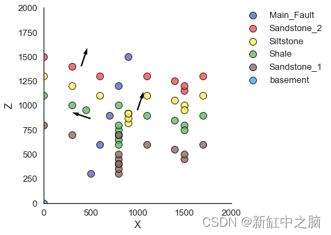
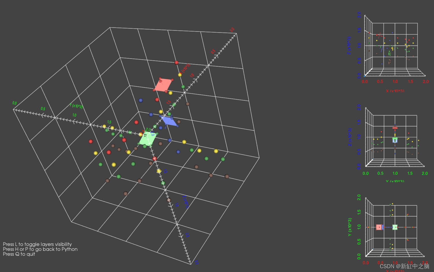
在这一部分中,使用 2D 和 3D 表示来呈现界面和方向。
gp.plot_data(geo_data, direction='y')

E:\Software\Anaconda3\lib\site-packages\gempy\gempy_front.py:927: FutureWarning: gempy plotting functionality will be moved in version 1.2, use gempy.plotting module instead
  warnings.warn("gempy plotting functionality will be moved in version 1.2, use gempy.plotting module instead", FutureWarning)
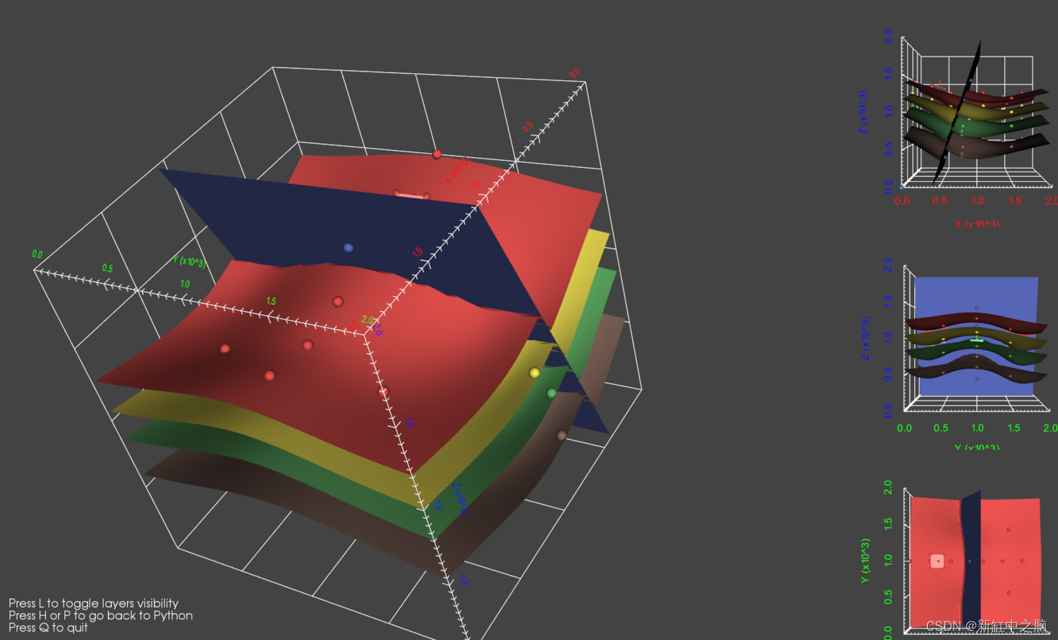
gp.plotting.plot_data_3D(geo_data)
6、地质插值
输入数据准备好后,我们可以使用 Gempy 库中的 InterpolatonData 方法定义插值的数据和参数。
地质模型是在“compute_model”方法下计算的。 模型过程的结果是与 geo_data 具有相同阵列维度的岩性和断层。
interp_data = gp.InterpolatorData(geo_data, u_grade=[1,1], output='geology', compile_theano=True, theano_optimizer='fast_compile')

Compiling theano function...
Compilation Done!
Level of Optimization:  fast_compile
Device:  cpu
Precision:  float32
Number of faults:  1

interp_data.geo_data_res.formations.as_matrix

<bound method NDFrame.as_matrix of              value  formation_number
Main_Fault       1                 1
Sandstone_2      2                 2
Siltstone        3                 3
Shale            4                 4
Sandstone_1      5                 5
basement         6                 6>

interp_data.geo_data_res.get_formations()

[Main_Fault, Sandstone_2, Siltstone, Shale, Sandstone_1]
Categories (5, object): [Main_Fault, Sandstone_2, Siltstone, Shale, Sandstone_1]

lith_block, fault_block = gp.compute_model(interp_data)
7、岩性模型勘探
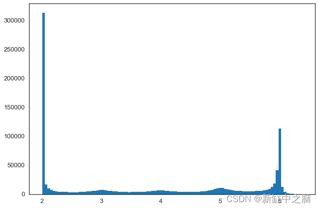
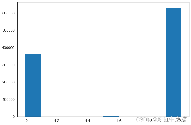
岩性块有两部分,第一部分包含有关岩性地层的信息,第二部分表示方向。 在这部分中,岩性和断层分离信息的分布以直方图的形式表示。
lith_block[0]

array([ 6.3131361 ,  6.24877167,  6.19397354, ...,  2.00398016,
        2.00626612,  2.00983   ], dtype=float32)

plt.hist(lith_block[0],bins=100)
plt.show()
plt.hist(fault_block[0],bins=10)
plt.show()
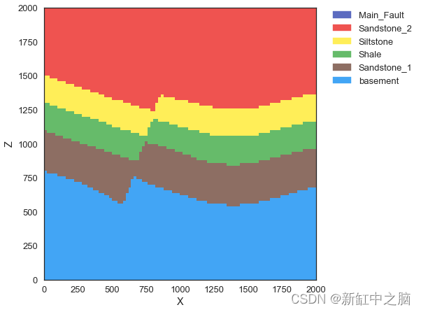
8、地质模型表示
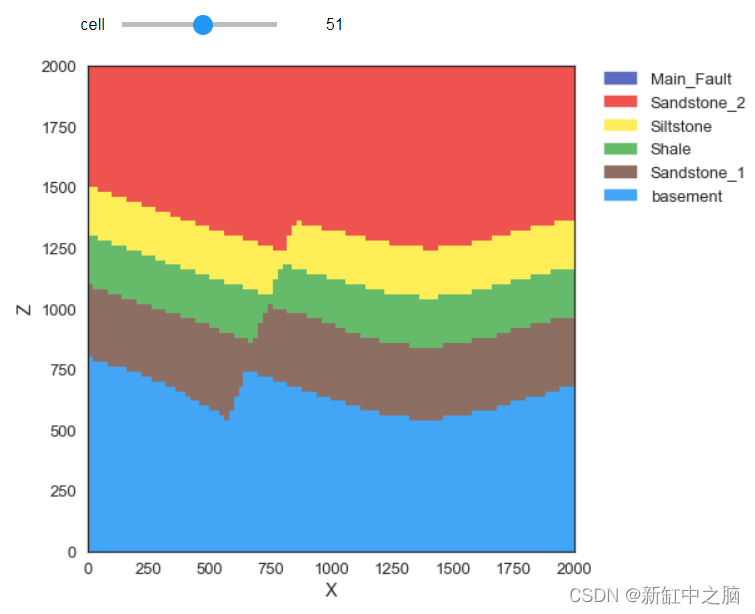
与任何其他 Numpy 数组一样,生成的岩性块可以在 Matplotlib 上表示。 然而,Gempy 有特殊的横截面表示方法。 通过使用 Jupyter 小部件,可以使用手柄沿行移动来执行沿 Y 方向的地质横截面的交互式表示。
gp.plotting.plot_section(geo_data, lith_block[0], cell_number=50, direction='y', plot_data=False)
import ipywidgets as widgets

def plotCrossSection(cell):
    gp.plotting.plot_section(geo_data, lith_block[0], cell_number=cell,  direction='y', plot_data=False)


widgets.interact(plotCrossSection,
cell=widgets.IntSlider(min=0,max=99,step=1,value=50) )
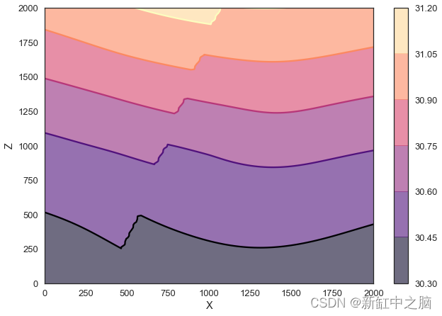
gp.plotting.plot_scalar_field(geo_data, lith_block[1], cell_number=50, N=6,
                        direction='y', plot_data=False)
plt.colorbar()
plt.show()
ver_s, sim_s = gp.get_surfaces(interp_data,lith_block[1],
                               fault_block[1],
                               original_scale=True)

gp.plotting.plot_surfaces_3D(geo_data, ver_s, sim_s)