人工智能系列实验（一）——用于识别猫的二分类单层神经网络

本实验利用Python，搭建了一个用于识别猫的单神经元神经网络，最终实现在测试集上的准确率在70%以上。

实验环境： python中numpy、matplotlib、h5py和skimage库

import numpy as np
import matplotlib.pyplot as plt  # 用于画图
import h5py  # 用于加载训练数据集
import skimage.transform as tf  # 用于缩放图片

训练样本： 209张64*64的带标签图片

测试样本： 50张64*64的带标签图片

关于本实验中所用数据集与完整代码详见：
https://github.com/PPPerry/AI_projects/tree/main/1.cats_identification

构建的神经网络模型如下：

在这里插入图片描述

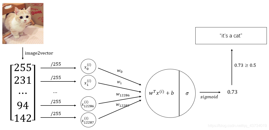
基于该神经网络模型，代码实现如下：

首先，对数据集数据进行预处理。

def load_dataset():
    """
    加载数据集数据
    :return: 训练数据与测试数据的相关参数
    """
    train_dataset = h5py.File("datasets/train_catvnoncat.h5", "r")
    train_set_x_orig = np.array(train_dataset["train_set_x"][:])  # 提取训练数据的特征数据，格式为(样本数, 图片宽, 图片长, 3个RGB通道)
    train_set_y_orig = np.array(train_dataset["train_set_y"][:])  # 提取训练数据的标签数据，格式为(样本数, )

    test_dataset = h5py.File("datasets/test_catvnoncat.h5", "r")
    test_set_x_orig = np.array(test_dataset["test_set_x"][:])  # 提取测试数据的特征数据
    test_set_y_orig = np.array(test_dataset["test_set_y"][:])  # 提取测试数据的标签数据

    classes = np.array(test_dataset["list_classes"][:])  # 提取标签，1代表是猫，0代表不是猫

    train_set_y_orig = train_set_y_orig.reshape((1, train_set_y_orig.shape[0]))  # 统一类别数组格式为(1, 样本数)
    test_set_y_orig = test_set_y_orig.reshape((1, test_set_y_orig.shape[0]))

    return train_set_x_orig,  train_set_y_orig, test_set_x_orig, test_set_y_orig, classes


train_set_x_orig,  train_set_y, test_set_x_orig, test_set_y, classes = load_dataset()  # 加载数据集数据

m_train = train_set_x_orig.shape[0]  # 训练样本数
m_test = test_set_x_orig.shape[0]  # 测试样本数
num_px = test_set_x_orig.shape[1]  # 正方形图片的长/宽

train_set_x_flatten = train_set_x_orig.reshape(train_set_x_orig.shape[0], -1).T  # 将样本数据进行扁平化和转置，格式为(图片数据, 样本数)
test_set_x_flatten = test_set_x_orig.reshape(test_set_x_orig.shape[0], -1).T

train_set_x = train_set_x_flatten/255.  # 标准化处理，使所有值都在[0, 1]范围内
test_set_x = test_set_x_flatten/255.

其次，构造神经网络中用到的相应函数。
其中，前向传播的公式为
$\begin{array}{c} A=\sigma(w^TX+b)=(a^{(1)},a^{(2)},\cdots,a^{(m-1)},a^{(m)})\\ \\ J = -\frac{1}{m}\sum^m_{i=1}log(a^{(i)})+(1-y^{(i)})log(1-a^{(i)}) \end{array}$
反向传播的公式为
$\begin{array}{c} \frac{\partial J}{\partial w} = \frac{1}{m}X(A-Y)^T\\ \\ \frac{\partial J}{\partial b} = \frac{1}{m}\sum^m_{i=1}(a^{(i)}-y^{(i)}) \end{array}$

def sigmoid(z):
    """
    sigmod函数实现
    :param z: 数值或一个numpy数组
    :return: [0, 1]范围数值
    """
    s = 1 / (1 + np.exp(-z))
    return s


def initialize_with_zeros(dim):
    """
    初始化权重数组w和偏置b为0
    :param dim: 权重值的数量
    :return:
    w: 权重数组
    b: 偏置bias
    """
    w = np.zeros((dim, 1))
    b = 0
    return w, b


def propagate(w, b, X, Y):
    """
    实现正向传播和反向传播，分别计算出成本与梯度
    :param w: 权重数组
    :param b: 偏置
    :param X: 图片的特征数据
    :param Y: 图片的标签数据
    :return:
    cost: 成本
    dw: w的梯度
    db：b的梯度
    """
    m = X.shape[1]

    # 前向传播
    A = sigmoid(np.dot(w.T, X) + b)
    cost = -np.sum(Y * np.log(A) + (1 - Y) * np.log(1 - A)) / m

    # 反向传播
    dZ = A - Y
    dw = np.dot(X, dZ.T) / m
    db = np.sum(dZ) / m

    # 梯度保存在字典中
    grads = {
    
    
        "dw": dw,
        "db": db
    }

    return grads, cost


def optimize(w, b, X, Y, num_iterations, learning_rate, print_cost=False):
    """
    梯度下降算法更新参数
    :param w: 权重数组
    :param b: 偏置bias
    :param X: 图片的特征数据
    :param Y: 图片的标签数据
    :param num_iterations: 优化迭代次数
    :param learning_rate: 学习率
    :param print_cost: 为真时，每迭代100次，打印一次成本
    :return:
    params: 优化后的w和b
    costs: 每迭代100次，记录一次成本
    """
    costs = []

    for i in range(num_iterations):
        grads, cost = propagate(w, b, X, Y)

        dw = grads["dw"]
        db = grads["db"]

        # 梯度下降
        w = w - learning_rate * dw
        b = b - learning_rate * db

        # 记录成本变化
        if i % 100 == 0:
            costs.append(cost)
            if print_cost:
                print("优化%d次后成本是：%f" % (i, cost))

    params = {
    
    
        "w": w,
        "b": b
    }

    return params, costs


def predict(w, b, X):
    """
    预测函数，判断是否为猫
    :param w: 权重数组
    :param b: 偏置bias
    :param X: 图片的特征数据
    :return:
    Y_predicition: 预测是否为猫，返回值为0或1
    p: 预测为猫的概率
    """
    m = X.shape[1]
    Y_prediction = np.zeros((1, m))

    p = sigmoid(np.dot(w.T, X) + b)

    for i in range(p.shape[1]):
        if p[0, i] >= 0.5:
            Y_prediction[0, i] = 1

    return Y_prediction, p

最终，组合以上函数，构建出最终的神经网络模型函数。

def model(X_train, Y_train, X_test, Y_test, num_iterations=2001, learning_rate=0.5, print_cost=False):
    """
    最终的神经网络模型函数
    :param X_train: 训练样本的特征数据
    :param Y_train: 训练样本的标签数据
    :param X_test: 测试样本的特征数据
    :param Y_test: 测试样本的标签数据
    :param num_iterations: 优化迭代次数
    :param learning_rate: 学习率
    :param print_cost: 为真时，每迭代100次，打印一次成本
    :return:
    d: 返回相关信息的字典
    """
    w, b = initialize_with_zeros(X_train.shape[0])  # 初始化参数

    parameters, costs = optimize(w, b, X_train, Y_train, num_iterations, learning_rate, print_cost)  # 训练参数
    w = parameters["w"]
    b = parameters["b"]

    Y_prediction_train, p_train = predict(w, b, X_train)
    Y_prediction_test, p_test = predict(w, b, X_test)

    print("对训练数据的预测准确率为：{}%".format(100 - np.mean(np.abs(Y_prediction_train - Y_train)) * 100))
    print("对测试数据的预测准确率为：{}%".format(100 - np.mean(np.abs(Y_prediction_test - Y_test)) * 100))

    d = {
    
    
        "costs": costs,
        "Y_prediction_test": Y_prediction_test,
        "Y_prediction_train": Y_prediction_train,
        "w": w,
        "b": b,
        "learning_rate": learning_rate,
        "num_iterations": num_iterations,
        "p_train": p_train,
        "p_test": p_test
    }

    return d

现在调用上面的模型函数对我们最开始加载的数据进行训练。

d = model(train_set_x, train_set_y, test_set_x, test_set_y, num_iterations=2001, learning_rate=0.005, print_cost=True)

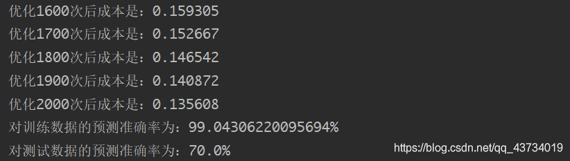
输出：优化2000次后的成本是0.1356。对训练数据的准确率为99%左右，对测试数据的准确率为70%左右。
在这里插入图片描述

试验模型预测功能：

查看训练集和测试集中图片及其对应的预测结果

def show_predict(index, prediction=np.hstack((d["Y_prediction_train"], d["Y_prediction_test"])),
                 data=np.hstack((train_set_x, test_set_x)), origin=np.hstack((train_set_y, test_set_y)),
                 px=num_px, p=np.hstack((d["p_train"], d["p_test"]))):
    if index >= prediction.shape[1]:
        print("index超出数据范围")
        return
    plt.imshow(data[:, index].reshape((px, px, 3)))
    plt.show()
    print("这张图的标签是" + str(origin[0, index]) + "，预测分类是" + str(int(prediction[0, index])) + "，预测概率是" + str(p[0, index]))

    return

以第19张图片为例：
在这里插入图片描述
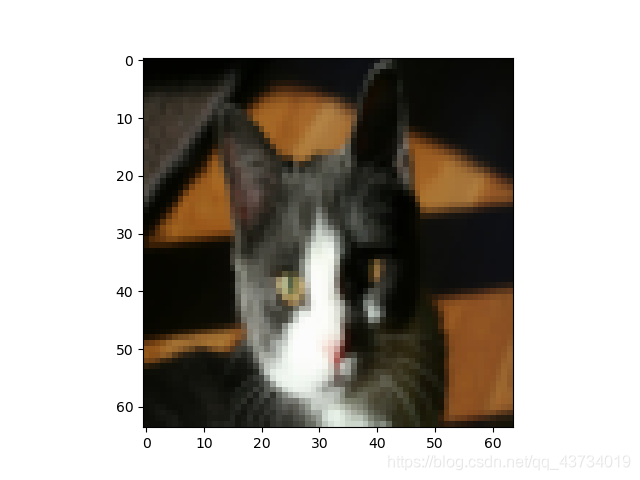
输出：这张图的标签是1，预测分类是1，预测概率是0.93。

扫描二维码关注公众号，回复： 15692814 查看本文章

查看自己输入的图片及其对应的预测结果

# 预测自己的图片
# 在同目录下创建一个文件夹images,把你的任意图片改名成my_image1.jpg后放入文件夹
my_image = "my_image1.jpg"

image = np.array(plt.imread(my_image))
my_image = tf.resize(image, (num_px, num_px), mode='reflect').reshape((1, num_px*num_px*3)).T
my_prediction, my_p = predict(d["w"], d["b"], my_image)

plt.imshow(image)
plt.show()
print("预测分类是" + str(int(my_prediction[0, 0])) + "，预测概率是" + str(my_p[0, 0]))

以下图为例：
在这里插入图片描述
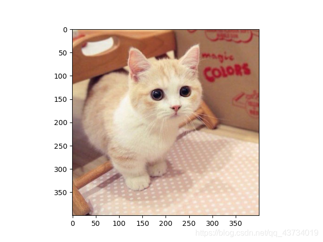
输出：预测分类是1，预测概率是0.89。

进一步实验得到的结论：

成本随迭代次数增加时的变化情况

# 绘制成本随迭代次数增加时的变化情况
costs = np.squeeze(d['costs'])  # 将表示向量的数组转换为秩为1的数组，便于matplotlib库函数画图
plt.plot(costs)
plt.ylabel('cost')
plt.xlabel('iterations (per hundreds)')
plt.title("Learning rate =" + str(d["learning_rate"]))
plt.show()

在这里插入图片描述
结论：训练次数越多，成本越小，预测结果越精确。

不同学习率下成本随迭代次数增加时的变化情况

# 绘制在不同学习率下成本随迭代次数增加时的变化情况
learning_rates = [0.01, 0.001, 0.0001]
models = {
    
    }
for i in learning_rates:
    models[str(i)] = model(train_set_x, train_set_y, test_set_x, test_set_y, num_iterations=2001, learning_rate=i,
                           print_cost=False)

for i in learning_rates:
    plt.plot(np.squeeze(models[str(i)]["costs"]), label=str(models[str(i)]["learning_rate"]))

plt.ylabel('cost')
plt.xlabel('iterations (per hundreds)')
legend = plt.legend(loc='upper right', shadow=True)
plt.show()

在这里插入图片描述
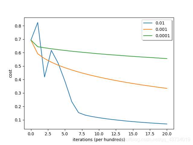
结论：选择一个正确的学习率很重要，不一定越大越好。设置不合理，神经网络有可能永远都不能下降到损失函数的最小值处；相反，设置合理，可以使神经网络的收敛达到很好的效果。

结束语：

实验过程中，一定要搞清楚变量的维度，否则做数据处理、写数组操作时会容易出现问题。
数据集、图片等需要和代码在同一目录下。
本实验几乎基于纯Python的numpy库函数进行神经网络模型的搭建，没有使用任何机器学习框架，重在理解数学原理及意义。在后续的实验中，我会对TensorFlow等经典框架进行学习与运用。
相关代码可能会不断更新改进，以github中的代码为准。
这是我在系统学习人工智能中实现的第一个人工智能程序，后续还会不断更新系列实验。写博客以督促自己不能总摸鱼233，希望自己能在神经网络这条路上走的尽可能远一些。