！！！这篇不涉及实现，仅从官方代码了解一下输出处理的思路，有机会的话会做实现，照例放出官方代码地址和之前写的论文解读：

SGRN网络github项目地址https://github.com/simblah/SGRN_torch [图神经网络]空间关系感知关系网络(SGRN)-论文解读https://blog.csdn.net/weixin_37878740/article/details/129837774?spm=1001.2014.3001.5501

一、网络框架回顾

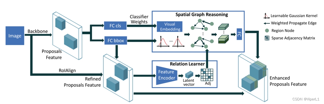
可以很明显的看到，论文提及的SGRN网络是在Faster R-CNN中嵌入了关系图学习器和空间感知推理模块，且将RoI Pooling改为RoI Align，故我们重点来看这几个部分的代码。

二、代码解读

所解读的代码位于项目的：lib->nets->network_gcn中。前向传递函数的结构如下：

    def forward(self, image, im_info, gt_boxes=None, mode='TRAIN'):
        #.....
        rois, cls_prob, bbox_pred = self._predict()
        #....

前向传递函数中其余代码均为数据预处理和损失函数计算，其次rois,cls_prob和bbox_pred均由self._predict( )函数计算得出。故跳转到_predict( )函数

# This is just _build_network in tf-faster-rcnn
net_conv = self._image_to_head()          #骨干网络提取

# build the anchors for the image
self._anchor_component(net_conv.size(2), net_conv.size(3))

rois = self._region_proposal(net_conv)    #获取候选区域
if cfg.POOLING_MODE == 'align':           #兴趣域池化
    pool5 = self._roi_align_layer(net_conv, rois)
else:
    pool5 = self._roi_pool_layer(net_conv, rois)

fc7 = self._head_to_tail(pool5)

cls_prob, bbox_pred = self._region_classification(fc7)

这是原属于Faster R-CNN的代码，修改了RoI Pooling，对应图示的这个部分：

1.RoI Align

def _roi_align_layer(self, bottom, rois):
    return RoIAlign((cfg.POOLING_SIZE, cfg.POOLING_SIZE), 1.0 / 16.0,0)(bottom, rois)

def _roi_pool_layer(self, bottom, rois):
    return RoIPool((cfg.POOLING_SIZE, cfg.POOLING_SIZE),1.0 / 16.0)(bottom, rois)

相较于RoI Pool，RoI Align最后多了一个参数，作用是控制双线性插值中采样点的个数，默认值为-1，代码中将其置为0。

2.关系学习器

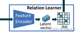
用于从权重中构建图（邻接矩阵），对应图示这个部分：

num_rois = rois.shape[0]    #通道数
z = self.relation_fc_1(fc7)
z = F.relu(self.relation_fc_2(z))
eps = torch.mm(z, z.t())
_, indices = torch.topk(eps, k=32, dim=0)

其中relation_fc_1()和relation_fc_2()均为全连接层，两个全连接层叠加后跟一个relu激活函数，fc7（即建议区域）经过模块处理后得到长度为256的序列z

self.relation_fc_1 = nn.Linear(self._fc7_channels, 256)
self.relation_fc_2 = nn.Linear(256, 256)

随后经过torch.mm( )<用途是将两个矩阵相乘>，将z与其转置相乘得到邻接矩阵eps。

邻接矩阵eps经过torch.topk( )，torch.topk的作用是找到序列中前k个元素进行排序，其返回值有两个：第一个值为排序的数组，第二个值为该数组中获取到的元素在原数组中的位置标号。这个函数的用途是用来构建稀疏图（对应原文取最大的3个值）。

排序规则为：该列最大的数据，以此类推：

tensor1=torch.tensor([  [9,1,2,1,9,1],
                        [3,4,5,1,1,1],
                        [7,8,9,1,1,1],
                        [1,4,7,1,1,2]])

values,indices=torch.topk(tensor1, k=3, dim=0)

print(values)
print(indices)

实验结果为，可以看到每一排最大的k个数据被提到了前面。

tensor([[9, 8, 9, 1, 9, 2],
        [7, 4, 7, 1, 1, 1],
        [3, 4, 5, 1, 1, 1]])

tensor([[0, 2, 2, 0, 0, 3],
        [2, 1, 3, 1, 1, 0],
        [1, 3, 1, 2, 2, 1]])

3.空间感知推理模块

①得到嵌入嵌入向量

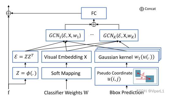
用于将图中的特征嵌入到图（邻接矩阵）中，对应图示这个部分：

具体结构如下，由三个分支组成（图/邻接矩阵，分类权重，预测框，分别代表：连接关系，类别关系，位置关系）

cls_w = self.cls_score_net.weight
represent = torch.mm(cls_prob, cls_w)

将cls_prob（分类器得出的类型预测权重）和cls_w（fc7经过一个线性分类器）相乘

self.cls_score_net = nn.Linear(self._fc7_channels, self._num_classes)

②得到距离函数

cls_pred = torch.max(cls_prob, 1)[1]
bbox_pred_reshape = bbox_pred.view(-1, 1001, 4)
bbox_pred_cls = torch.zeros(num_rois, 4)
for i, cls in enumerate(cls_pred):
    bbox_pred_cls[i] = bbox_pred_reshape[i][cls]
bbox_pred_ctr = bbox_pred_cls[:, 0:2] + bbox_pred_cls[:, 2:4]

torch.max()[1]返回的是最大值的索引，实验如下：

x = torch.max(tensor1,1)[1]    #tensor1同上例
print(x)

tensor([0, 2, 2, 2])    #得到每一列最大值的索引

bbox_pred是由关系分类器处理fc7后得到的目标框预测，使用view对其进行重构，然后遍历cls_pred，取出每列最大的元素（四个坐标）；再按照公式（如下）进行计算

$d=\sqrt{(c_a-c_b)^2+(y_a-y_b)^2}$ ， $\theta=arctan(\frac{y_b-y_a}{c_b-c_a})$

relation = torch.empty(2, 32 * num_rois, dtype=torch.long).to(self._device)
# U = torch.empty(32*128, 2).to(self._device)

relation[0] = torch.Tensor(list(range(num_rois)) * 32)  # , type=torch.long)
relation[1] = indices.view(-1)

coord_i = bbox_pred_ctr[relation[0]]
coord_j = bbox_pred_ctr[relation[1]]

d = torch.sqrt((coord_i[:, 0] - coord_j[:, 0]) ** 2 + (coord_i[:, 1] - coord_j[:, 1]) ** 2)
#距离
theta = torch.atan2((coord_j[:, 1] - coord_i[:, 1]), (coord_j[:, 0] - coord_i[:, 0]))
#角度

U = torch.stack([d, theta], dim=1).to(self._device)
#位置嵌入

③图卷积

图卷积的定义为，参数分别为：输入图尺寸，输出图尺寸，深度，卷积核尺寸

self.gaussian = GMMConv(self._fc7_channels, self._fc7_channels, dim=2, kernel_size = 25)

使用此图卷积处理：图/邻接矩阵，分类权重，预测框（三个输入实际分别为：图（graph）、特征（feat ）、伪坐标（pseudo），其中，特征/feat的尺寸为（ $N,D_{in}$ ）<分别表示：节点数量，输入特征的尺寸>；伪坐标/pseudo的尺寸为( $E,D_u$ )<分别表示：边的条数，伪坐标的维数>）

f = self.gaussian(represent, relation, U)

使用全连接和激活函数处理图嵌入：

f2 = F.relu(self.sg_conv_1(f))
h = F.relu(self.sg_conv_2(f2))

其中2个全连接sg_conv为：

self.sg_conv_1 = nn.Linear(self._fc7_channels, 512)
self.sg_conv_2 = nn.Linear(512, 256)

4.将图与候选区域融合

将图得到的嵌入向量和候选区域进行融合后得到新的预测框和分类数据

new_f = torch.cat([fc7, h], dim=1)
new_cls_prob, new_bbox_pred = self._new_region_classification(new_f)

for k in self._predictions.keys():
    self._score_summaries[k] = self._predictions[k]

return rois, new_cls_prob, new_bbox_pred

上面所用到的_new_region_classification( )的实现为：

def _new_region_classification(self, f):
    cls_score = self.new_cls_score_net(f)
    cls_pred = torch.max(cls_score, 1)[1]
    cls_prob = F.softmax(cls_score, dim=1)
    bbox_pred = self.new_bbox_pred_net(f)

    self._predictions["cls_score"] = cls_score
    self._predictions["cls_pred"] = cls_pred
    self._predictions["cls_prob"] = cls_prob
    self._predictions["bbox_pred"] = bbox_pred

    return cls_prob, bbox_pred

[图神经网络]空间关系感知关系网络(SGRN)-代码解析