0.基础知识
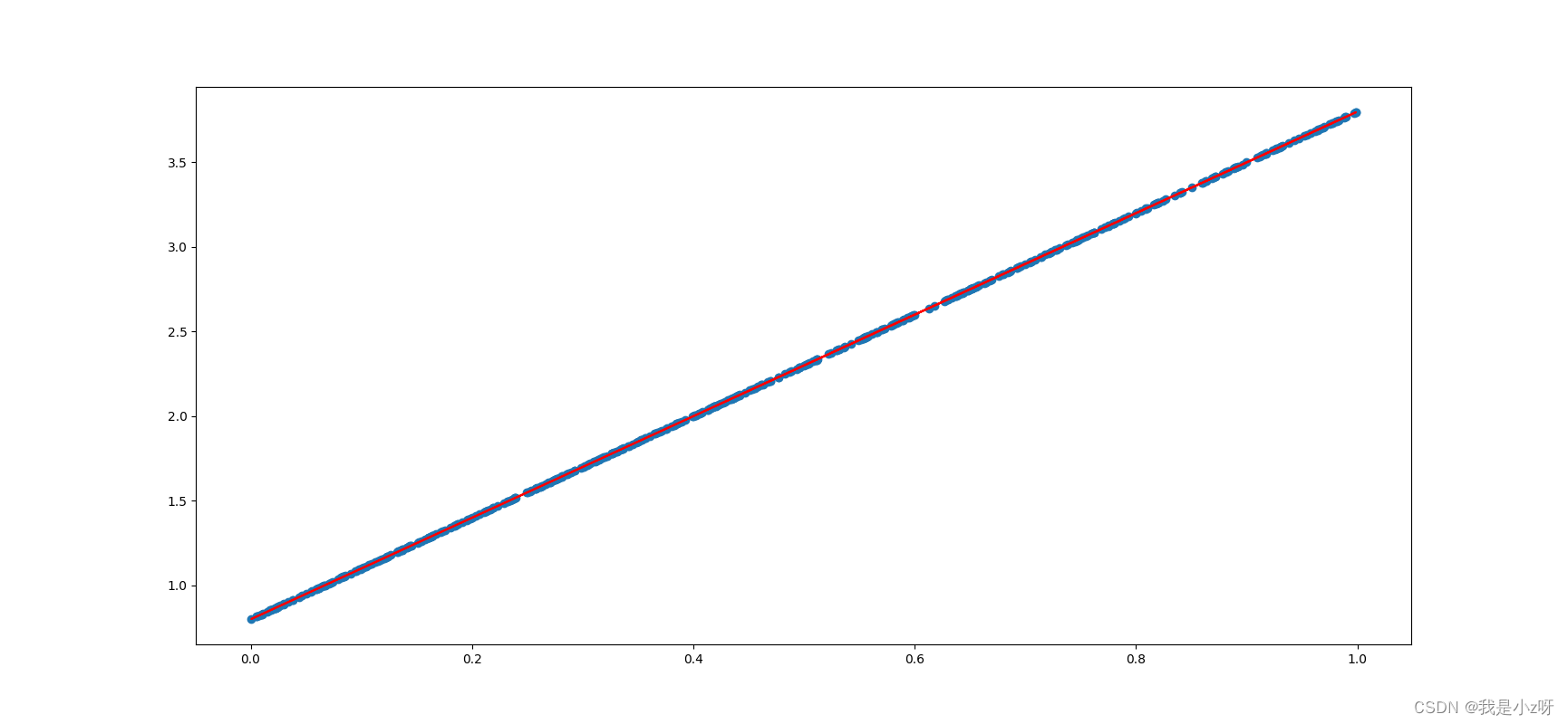
1.首先用pytorch手写一个线性回归,这里注意tensorflow是画静态图,所以 pred和loss写在循环外,但在torch里,是动态运行,所以写在循环体里。
import torch
import matplotlib.pyplot as plt
learning_rate=0.1
#1.准备数据y=3x+0.8
x=torch.rand([500,1])
y_true=x*3+0.8
w=torch.rand([1,1],requires_grad=True)
b=torch.tensor(0,requires_grad=True,dtype=torch.float32)
#2.根据loss反向传播更新参数
for i in range(2000):
    y_preidct=torch.matmul(x,w)+b
    loss=(y_true-y_preidct).pow(2).mean()
    if w.grad is not None:#每次反向传播前,梯度置为0,不然会累加梯度
        w.grad.data.zero_()
    if b.grad is not None:
        b.grad.data.zero_()
    loss.backward()
    w.data=w.data-learning_rate*w.grad
    b.data=b.data-learning_rate*b.grad
    if i%100==0:
        print("w,b,loss",w.item(),b.item(),loss.item())
#3.画图显示
plt.figure(figsize=(20,8))
plt.scatter(x.numpy().reshape(-1),y_true.numpy().reshape(-1))
y_preidct=torch.matmul(x,w)+b
plt.plot(x.numpy().reshape(-1),y_preidct.detach().numpy().reshape(-1),c='r')
plt.show()
2.用pytorch的api写线性回归
import torch
import torch.nn as nn
from torch.optim import SGD
device=torch.device("cuda" if torch.cuda.is_available() else "cpu")
#1.准备数据
x=torch.rand([500,1]).to(device)
y_true=3*x+0.8
learning_rate=0.001
#2.定义自己的模型结构
class MyLinear(nn.Module):
    def __init__(self):#1.继承父类init,并定义自己模型结构
        super(MyLinear,self).__init__()
        self.linear=nn.Linear(1,1)#in_features,out_featuresm
    def forward(self,x):#2.模型前向传播的结构搭起来
        out=self.linear(x)
        return out
#3.实例化模型,实例化loss,实例化优化器
my_linear=MyLinear().to(device)
loss_fn=nn.MSELoss()
optimizer=SGD(my_linear.parameters(),learning_rate)
#4.梯度下降,循环更新模型参数
for i in range(20000):
    y_predict=my_linear(x)#1.前向传播,拿到预测结果
    loss=loss_fn(y_predict,y_true)#2.计算模型损失
    optimizer.zero_grad()#3.梯度置为0
    loss.backward()#4.反向传播
    optimizer.step()#5.参数更新
    if i%100==0:
        print("epoch[{}/{}],loss:{:.6f}".format(i,20000,loss.data))
3.使用pytorch的数据集类和数据加载器类处理自己的数据集。
import torch
from torch.utils.data import Dataset,DataLoader
#1.继承使用torch的数据集类,来处理自己的数据
class SmsDataset(Dataset):
    def __init__(self):#1.初始化,获取自己数据
        self.file_path=r"./Data/SMSSpamCollection"
        self.lines=open(self.file_path).readlines()
    def __getitem__(self,index):#2.getitem获取索引位置的一条数据
        line=self.lines[index].strip()
        label=line.split("\t")[0]
        content=line.split("\t")[1]
        return label,content
    def __len__(self):#3.获取数据总长
        return len(self.lines)
sms_dataset=SmsDataset()
#2.继承使用torch的数据加载器类,进行数据规定格式的加载
dataloader=DataLoader(sms_dataset,batch_size=4,shuffle=True,drop_last=True)
#3.使用这两个类得出需要的批数据
if __name__=="__main__":
    for idx,(labels,contents) in enumerate(dataloader):
        print(idx)
        print(labels)
        print(contents)
        break
    print(len(sms_dataset))
    print(len(dataloader))
4.pytorch自带的数据集,torchvision.datasets里面是一些图像数据集;torchtext.datasets里面是一些文本数据集。下面是使用图像数据集的mnist进行手写图像识别。其中需要三个api来对数据进行处理。
torchvision.transforms.ToTensor():把image对象或者(h,w,c)转化为(c,h,w)
torchvision.transforms.Normalize(mean,std):均值和标准差的形状和通道数相同
torchvision.transforms.Compose(transforms):传入list,数据经过list中的每一个方法挨个进行处理。
import torch
from torch.utils.data import DataLoader
from torchvision.datasets import MNIST
import torchvision
import torch.nn as nn
import torch.nn.functional as F
from torch import optim
from tqdm import tqdm
import numpy as np
import os
train_batch_size=128
test_batch_size=1000
device=torch.device("cuda" if torch.cuda.is_available() else "cpu")
#1.准备数据
def mnist_dataset(train):#1.数据集类处理
    func=torchvision.transforms.Compose([torchvision.transforms.ToTensor(),torchvision.transforms.Normalize(mean=(0.1307),std=(0.3081))])
    return MNIST(root="./Data/mnist",train=train,download=True,transform=func)
def get_dataloader(train=True):#2.数据加载器类处理
    mnist=mnist_dataset(train)
    batch_size=train_batch_size if train else test_batch_size
    return DataLoader(mnist,batch_size=batch_size,shuffle=True)
#2.搭模型结构
class MnistModel(nn.Module):
    def __init__(self):
        super(MnistModel,self).__init__()
        self.fc1=nn.Linear(1*28*28,100)#输入,输出
        self.fc2=nn.Linear(100,10)
    def forward(self,image):
        image_view=image.view(-1,1*28*28)#[batch_size,1*28*28]
        fc1_out=self.fc1(image_view)
        fc1_out_relu=F.relu(fc1_out)
        out=self.fc2(fc1_out_relu)
        return F.log_softmax(out,dim=-1)
#3.训练并保存模型
model=MnistModel().to(device)
optimizer=optim.Adam(model.parameters(),lr=1e-2)
def train(epoch):
    train_data=get_dataloader(train=True)
    bar=tqdm(enumerate(train_data),total=len(train_data))
    total_loss=[]
    for idx,(input,target) in bar:
        input=input.to(device)
        target=target.to(device)
        optimizer.zero_grad()#梯度置为0
        output=model(input)
        loss=F.nll_loss(output,target)
        loss.backward()
        total_loss.append(loss.item())
        optimizer.step()#参数更新
        if idx%100==0:
            bar.set_description("epoch{} idx:{},loss:{:.6f}".format(epoch,idx,np.mean(total_loss)))
            torch.save(model.state_dict(),"./Models/model.pkl")
            torch.save(optimizer.state_dict(),"./Models/optimizer.pkl")
#4.评估测试模型
def eval():
    model=MnistModel().to(device)
    if os.path.exists("./Models/model.pkl"):
        model.load_state_dict(torch.load("./Models/model.pkl"))
    test_data=get_dataloader(train=False)
    total_loss=[]
    total_acc=[]
    with torch.no_grad():#评估时不更新参数
        for input,target in test_data:#分batch拿数据
            input = input.to(device)
            target = target.to(device)
            output = model(input)
            loss = F.nll_loss(output,target)
            total_loss.append(loss.item())
            pred = output.max(dim=-1)[-1]
            total_acc.append(pred.eq(target).float().mean().item())
    print("test loss:{},test acc:{}".format(np.mean(total_loss),np.mean(total_acc)))
if __name__ == '__main__':
    #for i in range(10):
     #    train(i)
    eval()
5.文本情感分类,第一步(数据.py)是在建造数据与向量的映射,并把train里面的分词和向量映射以及特殊字符映射建造一个字典,并建立数据器和数据加载器。
#首先拿到数据进行tokenize,然后转换成torch输入类型的数据
from torch.utils.data import Dataset,DataLoader
import torch
import os
import re
import pickle
import tqdm
train_batch_size=512
test_batch_size=500
max_len=50
# ws=pickle.load(open("./models/ws.pkl","rb"))
#1.继承数据集类,对句子分词
def tokenize(sentence):#将每个句子里面的特殊字符都替换成空格并进行分词
    sentence=re.sub("<.*?>"," ",sentence)
    filters=['!', '"', '#', '$', '%', '&', '\(', '\)', '\*', '\+', ',', '-', '\.', '/', ':', ';', '<', '=', '>',
                '\?', '@', '\[', '\\', '\]', '^', '_', '`', '\{', '\|', '\}', '~', '\t', '\n', '\x97', '\x96', '”', '“', ]
    sentence = re.sub("|".join(filters)," ",sentence)
    sentence = sentence.lower()
    result = [i for i in sentence.split(" ")if len(i)>0]
    return result
class ImdbDataset(Dataset):#继承数据集类
    def __init__(self,train=True):#拿到每个txt的地址
        self.data_path=r"\\Mac\Home\Desktop\JOB\gpt\Data\aclImdb_v1"
        self.data_path+=r'\train' if train else r"\test"
        self.total_path=[]
        for temp in [r"\pos",r"\neg"]:
            cur_path=self.data_path+temp
            self.total_path+=[os.path.join(cur_path,i) for i in os.listdir(cur_path) if i.endswith(".txt")]
    def __getitem__(self,idx):#每句话进行分词,并把标签做二分类
        file=self.total_path[idx]
        review=tokenize(open(file, encoding="utf8").read())
        label=int(file.split("_")[-1].split(".")[0])
        label =0 if label<5 else 1
        return review,label
    def __len__(self):
        return len(self.total_path)
#2.词语进行序列化,并标识特殊字符
class WordSequence:
    PAD_TAG="<TAG>"
    UNK_TAG="<UNK>"
    PAD=0
    UNK=1
    def __init__(self):
        self.dict={

    self.UNK_TAG:self.UNK,self.PAD_TAG:self.PAD}
        self.count={

    }
    def fit(self,sentence):
        for word in sentence:
            self.count[word]=self.count.get(word,0)+1
    def build_vocab(self,min_count=5,max_count=2000,max_features=30000):#根据条件构造 词典
        """
        :param min_count:最小词频
        :param max_count: 最大词频
        :param max_features: 最大词语数
        """
        if min_count is not None:
            self.count={

    word:count for word,count in self.count.items() if count >= min_count}
        if max_count is not None:
            self.count={

    word:count for word,count in self.count.items() if count <= max_count}
        if max_features is not None:
            self.count = dict(sorted(self.count.items(),reverse=True)[:max_features])
        for word in self.count:
            self.dict[word]=len(self.dict)
        self.inverse_dict = dict(zip(self.dict.values(),self.dict.keys()))#把dict进行翻转
        return self.inverse_dict
    def transform(self,sentence,max_len=None):#把句子转化为数字序列
        if len(sentence)>max_len:
            sentence=sentence[:max_len]#裁剪
        else:
            sentence = sentence + [self.PAD_TAG] *(max_len- len(sentence))  #填充PAD
        return [self.dict.get(i,1) for i in sentence]#没有的tokenize为unk
    def inverse_transform(self,incides):#把数字序列转化为字符
        return [self.inverse_dict.get(i,"<UNK>") for i in incides]#没有的转化为unk
    def __len__(self):
        return len(self.dict)
#3.继承数据加载器类,对batch数据进行处理
def collate_fn(batch):
    reviews,labels = list(zip(*batch))
    reviews = torch.LongTensor([ws.transform(i,max_len=max_len) for i in reviews])
    labels = torch.LongTensor(labels)
    return reviews,labels
def get_dataloader(train=True):
    dataset = ImdbDataset(train)
    batch_size = train_batch_size if train else test_batch_size
    return DataLoader(dataset,batch_size=batch_size,shuffle=True,collate_fn=collate_fn)
if __name__ == '__main__':
    ws=WordSequence()
    train_data = ImdbDataset(train=True)
    for i in train_data.total_path :
        sentence=tokenize(open(i, encoding="utf8").read())#拿到了train里面已经分词的每个文本数据
        ws.fit(sentence)#词与数的映射
    ws.build_vocab()#根据映射和字典的词频等要求建字典
    print(len(ws))#30002
    pickle.dump(ws, open(r"\\Mac\Home\Desktop\JOB\gpt\5.文本情感分类\results\word_dict.pkl", "wb"))
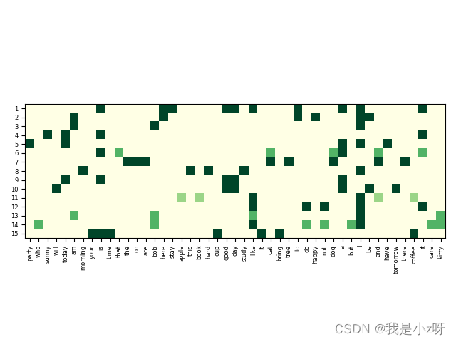
1. TF-IDF
搜索引擎中常用的技术方法,Term Frequency - Inverse Document Frequency (TF-IDF),是一种基于统计学的方法。这里我学习了莫烦的NLP课程。所以用numpy先实现以下。
import numpy as np
from collections import Counter
import matplotlib.pyplot as plt
import os
import itertools
def show_tfidf(tfidf, vocab, filename):
    # [n_doc, n_vocab]
    plt.imshow(tfidf, cmap="YlGn", vmin=tfidf.min(), vmax=tfidf.max())
    plt.xticks(np.arange(tfidf.shape[1]), vocab, fontsize=6, rotation=90)
    plt.yticks(np.arange(tfidf.shape[0]), np.arange(1, tfidf.shape[0]+1), fontsize=6)
    plt.tight_layout()
    # creating the output folder
    output_folder = './visual/results/'
    os.makedirs(output_folder, exist_ok=True)
    plt.savefig(os.path.join(output_folder, '%s.png') % filename, format="png", dpi=500)
    plt.show()
docs=["it is a good day, I like to stay here",
    "I am happy to be here",
    "I am bob",
    "it is sunny today",
    "I have a party today",
    "it is a dog and that is a cat",
    "there are dog and cat on the tree",
    "I study hard this morning",
    "today is a good day",
    "tomorrow will be a good day",
    "I like coffee, I like book and I like apple",
    "I do not like it",
    "I am kitty, I like bob",
    "I do not care who like bob, but I like kitty",
    "It is coffee time, bring your cup"]
#TF计算方法,TF显示文档d中词w的频率,这里提供了四种计算方法;idf方法,三种
def safe_log(x):
    mask=x!=0
    x[mask]=np.log(x[mask])
    return x
tf_methods={

    "log":lambda x:np.log(1+x),
            "augmented":lambda x:0.5+0.5*x/np.max(x,axis=1,keepdims=True),
            "boolean":lambda x:np.minium(x,1),
            "log_avg":lambda x:(1+safe_log(x)/(1+safe_log(np.mean(x,axis=1,keepdims=True))))}
idf_methods={

    "log":lambda x:1+np.log(len(docs)/(x+1)),
             "prob":lambda x:np.maximum(0,np.log((len(docs)-x)/(x+1))),#smooth平滑处理
             "len_norm":lambda x:x/(np.sum(np.square(x))+1)}
#1.文档的单词转换成ID形式
docs_words=[d.replace(",","").split() for d in docs]
vocab = set(itertools.chain(*docs_words))
v2i={

    v:i for i,v in enumerate(vocab)}
i2v={

    i:v for v,i in v2i.items()}
#2.开始计算TF和ITF值
def get_tf(method="log"):
    _tf=np.zeros((len(vocab),len(docs)),dtype=np.float64)#[词个数,文章个数]
    for i,d in enumerate(docs_words):
        counter=Counter(d)
        # print(counter)
        for v in counter.keys():
            # print(counter.most_common(1)[0][1])
            _tf[v2i[v],i]=counter[v]/counter.most_common(1)[0][1]
    weighted_tf=tf_methods.get(method,None)
    if weighted_tf is None:
        raise ValueError
    return weighted_tf(_tf)
def get_idf(method='log'):
    # print(i2v)
    df = np.zeros((len(i2v), 1))#[[词个数]]
    # print(df)
    for i in range(len(i2v)):
        d_count=0
        for d in docs_words:
            d_count+=1 if i2v[i] in d else 0
        df[i, 0] = d_count
    idf_fn=idf_methods.get(method,None)
    if idf_fn is None:
        raise ValueError
    return idf_fn(df)
#3.计算q和tfidf的余弦相似度
def cosine_similarity(q, _tf_idf):
    unit_q = q / np.sqrt(np.sum(np.square(q), axis=0, keepdims=True))
    unit_ds = _tf_idf / np.sqrt(np.sum(np.square(_tf_idf), axis=0, keepdims=True))
    similarity = unit_ds.T.dot(unit_q).ravel()
    return similarity
def docs_score(q, len_norm=False):
    q_words = q.replace(",", "").split(" ")

    # add unknown words
    unknown_v = 0
    for v in set(q_words):
        if v not in v2i:
            v2i[v] = len(v2i)
            i2v[len(v2i)-1] = v
            unknown_v += 1
    if unknown_v > 0:
        _idf = np.concatenate((idf, np.zeros((unknown_v, 1), dtype=np.float64)), axis=0)
        _tf_idf = np.concatenate((tf_idf, np.zeros((unknown_v, tf_idf.shape[1]), dtype=np.float64)), axis=0)
    else:
        _idf, _tf_idf = idf, tf_idf
    counter = Counter(q_words)
    q_tf = np.zeros((len(_idf), 1), dtype=np.float64)     # [n_vocab, 1]
    for v in counter.keys():
        q_tf[v2i[v], 0] = counter[v]
    q_vec = q_tf * _idf            # [n_vocab, 1]
    q_scores = cosine_similarity(q_vec, _tf_idf)
    if len_norm:
        len_docs = [len(d) for d in docs_words]
        q_scores = q_scores / np.array(len_docs)
    return q_scores
def get_keywords(n=2):
    for c in range(3):
        col = tf_idf[:, c]
        idx = np.argsort(col)[-n:]
        # print("doc{}, top{} keywords {}".format(c, n, [i2v[i] for i in idx]))
tf = get_tf()           # [n_vocab, n_doc]
idf = get_idf()         # [n_vocab, 1]
tf_idf = tf * idf       # [n_vocab, n_doc]
# print("tf shape(vecb in each docs): ", tf.shape)
# print("\ntf samples:\n", tf[:2])
# print("\nidf shape(vecb in all docs): ", idf.shape)
# print("\nidf samples:\n", idf[:2])
# print("\ntf_idf shape: ", tf_idf.shape)
# print("\ntf_idf sample:\n", tf_idf[:2])
# test
get_keywords()
q = "I get a coffee cup"
scores = docs_score(q)
d_ids = scores.argsort()[-3:][::-1]
# print("\ntop 3 docs for '{}':\n{}".format(q, [docs[i] for i in d_ids]))
show_tfidf(tf_idf.T, [i2v[i] for i in range(tf_idf.shape[0])], "tfidf_matrix")
使用Sklearn内置的tfidf模块会提高运算效率,其中对稀疏矩阵进行了矩阵压缩,减少存储与运算。
from sklearn.feature_extraction.text import TfidfVectorizer
from sklearn.metrics.pairwise import cosine_similarity
import matplotlib.pyplot as plt
import numpy as np
import os
#1.数据
docs = [
    "it is a good day, I like to stay here",
    "I am happy to be here",
    "I am bob",
    "it is sunny today",
    "I have a party today",
    "it is a dog and that is a cat",
    "there are dog and cat on the tree",
    "I study hard this morning",
    "today is a good day",
    "tomorrow will be a good day",
    "I like coffee, I like book and I like apple",
    "I do not like it",
    "I am kitty, I like bob",
    "I do not care who like bob, but I like kitty",
    "It is coffee time, bring your cup",
]
#2.模型并训练(fit_transform)
vectorizer=TfidfVectorizer()
tf_idf=vectorizer.fit_transform(docs)
print("idf: ", [(n, idf) for idf, n in zip(vectorizer.idf_, vectorizer.get_feature_names_out())])
print("v2i: ", vectorizer.vocabulary_)
#3.测试(transform)
q = "I get a coffee cup"
qtf_idf = vectorizer.transform([q])
res = cosine_similarity(tf_idf, qtf_idf)
res = res.ravel().argsort()[-3:]#3个主题词
print("\ntop 3 docs for '{}':\n{}".format(q, [docs[i] for i in res[::-1]]))
#4.plot
def show_tfidf(tfidf, vocab, filename):
    # [n_doc, n_vocab]
    plt.imshow(tfidf, cmap="YlGn", vmin=tfidf.min(), vmax=tfidf.max())
    plt.xticks(np.arange(tfidf.shape[1]), vocab, fontsize=6, rotation=90)
    plt.yticks(np.arange(tfidf.shape[0]), np.arange(1, tfidf.shape[0]+1), fontsize=6)
    plt.tight_layout()
    # creating the output folder
    output_folder = './visual/results/'
    os.makedirs(output_folder, exist_ok=True)
    plt.savefig(os.path.join(output_folder, '%s.png') % filename, format="png", dpi=500)
    plt.show()
i2v = {

    i: v for v, i in vectorizer.vocabulary_.items()}
dense_tfidf = tf_idf.todense()
show_tfidf(dense_tfidf, [i2v[i] for i in range(dense_tfidf.shape[1])], "tfidf_sklearn_matrix")
传统的tfidf方法可以表示词语出现的重要程度,但不能表示上下文词语的相似度,因此引入了W2V和cbow方法
2.Word2Vec和CBOW
1.因为one-hot编码有维度灾难和不能表示词相似度这两个缺点,所以用多维度的向量表示词,一般向量是50~300维。主要有根据中心词V预测上下文词U的skip-gram(跳字模型)方法和根据U预测V的CBOW(Continuous bag-of-words model连续词袋)模型。
2.Gensim(generate similarity)是一个简单高效的自然语言处理Python库,用于抽取文档的语义主题(semantic topics)。Gensim的输入是原始的、无结构的数字文本(纯文本),内置的算法包括Word2Vec,FastText,潜在语义分析(Latent Semantic Analysis,LSA),潜在狄利克雷分布(Latent Dirichlet Allocation,LDA)等,通过计算训练语料中的统计共现模式自动发现文档的语义结构。这些算法都是非监督的,这意味着不需要人工输入——仅仅需要一组纯文本语料。一旦发现这些统计模式后,任何纯文本(句子、短语、单词)就能采用语义表示简洁地表达。
这种方法可以包含上下文词语的相似度信息,但每个词语的向量信息已经固定,所以不能处理上下文中一词多义的现象,而且这些对词语的处理忽略了文章的语言顺序信息,因此使用seq2seq方法来理解每个句子。