Manipulator Jacobian - A Brief Note

Thanks Mark W. Spong et al for their great work of Robot Modeling and Control.
Thanks Zexiang Li et al for their great work of A Mathematical Introduction to Robotic Manipulation.
Thanks John J. Craig for his great work of Introduction to Robotics - Mechanics and Control - 3rd Edition.

We assume that all the frames mentioned below are right-handed.

End-effector Velocity and Manipulator Jacobian

Let $g_{st}:Q\to SE(3)$ be the forward kinematics map for a manipulator. If the joints move along a path $\theta(t)\in Q$, then the end-effector traverses a path $g_{st}(\theta(t))\in SE(3)$. The instantaneous spatial velocity of the endeffector is given by the twist:

$$\widehat{V}_{st}^{s}=\dot{g}_{st}(\theta)g_{st}^{-1}(\theta)$$ By the chain rule,
$$\widehat{V}_{st}^{s}=\sum_{t=1}^{n}\left(\frac{\partial g_{st}}{\partial \theta_{i}}\dot{\theta}_{i}\right)g_{st}^{-1}(\theta)=\sum_{t=1}^{n}\left(\frac{\partial g_{st}}{\partial \theta_{i}}g_{st}^{-1}(\theta)\right)\dot{\theta}_{i}$$ It can be seen that the end-effector velocity is linearly related to the velocity of the individual joints. In twist coordinates, the equation above can be written as
$$V_{st}^{s}=J_{st}^{s}(\theta)\dot{\theta}$$ where
$$J_{st}^{s}(\theta)=\left[\left(\frac{\partial g_{st}}{\partial \theta_{1}}g_{st}^{-1}\right)^{\vee} \cdots \left(\frac{\partial g_{st}}{\partial \theta_{n}}g_{st}^{-1}\right)^{\vee}\right]$$ We call the matrix $J_{st}^{s}(\theta)\in\mathbb{R}^{6\times n}$ the spatial manipulator Jacobian. By utilizing the product of exponential formula, we can obtain a more explicit and elegant formula for $J_{st}^{s}$. Let $\hat{\xi}_{i}\in se(3)$ be unit twists,
$$\begin{split}\frac{\partial g_{st}}{\partial \theta_{i}}g_{st}^{-1} &= e^{\hat{\xi}_{1}\theta_{1}}\cdots e^{\hat{\xi}_{i-1}\theta_{i-1}}(\hat{\xi}_{i})e^{\hat{\xi}_{i}\theta_{i}}\cdots e^{\hat{\xi}_{n}\theta_{n}}g_{st}(0)g_{st}^{-1} \\ &= e^{\hat{\xi}_{1}\theta_{1}}\cdots e^{\hat{\xi}_{i-1}\theta_{i-1}}(\hat{\xi}_{i})e^{-\hat{\xi}_{i-1}\theta_{i-1}}\cdots e^{-\hat{\xi}_{1}\theta_{1}} \end{split}$$ and converting to twist coordinates,
$$\left(\frac{\partial g_{st}}{\partial \theta_{i}}g_{st}^{-1}\right)^{\vee}=\mathrm{Ad}_{\left(e^{\hat{\xi}_{1}\theta_{1}}\cdots e^{\hat{\xi}_{i-1}\theta_{i-1}}\right)}\xi_{i}$$ The spatial manipulator Jacobian becomes:
$$\begin{gather}J_{st}^{s}(\theta)=[\xi_{1},\xi_{2}',\dots, \xi_{n}' ] \\ \xi_{i}'=\mathrm{Ad}_{\left(e^{\hat{\xi}_{1}\theta_{1}}\cdots e^{\hat{\xi}_{i-1}\theta_{i-1}}\right)}\xi_{i} \end{gather}$$ $J_{st}^{s}(\theta):\mathbb{R}^{n}\to \mathbb{R}^{6}$ is a configuration-dependent matrix which maps joint velocities to end-effector velocities. Obviously, the contribution of the $i$-th joint velocity to the end-effector velocity is independent of the configuration of later joints in the chain. Thus, the $i$-th column of the spatial Jacobian is the $i$-th joint twist, transformed to the current manipulator configuration.

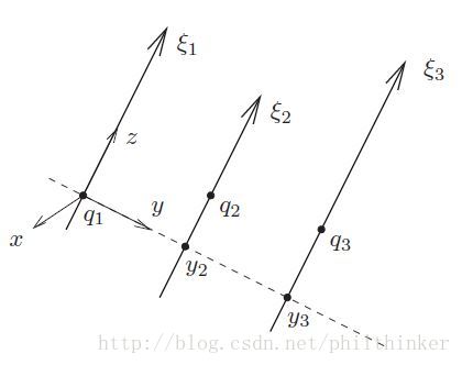
It is also possible to define a body manipulator Jacobian, $J^{b}_{st}$, which is defined by the relationship

$$V_{st}^{b}=J_{st}^{b}(\theta)\dot{\theta}$$ And
$$\begin{gather} J_{st}^{b}(\theta)=[\xi_{1}^{\dagger},\cdots , \xi_{n-1}^{\dagger}, \xi_{n}^{\dagger}] \\ \xi_{i}^{\dagger}=\mathrm{Ad}_{\left(e^{\hat{\xi}_{i}\theta_{i}}\cdots e^{\hat{\xi}_{n}\theta_{n}}g_{st}(0)\right)}^{-1}\xi_{i} \end{gather}$$ The columns of $J_{st}^{b}$ correspond to the joint twists written with respect to the tool frame at the current configuration. Note that $g_{st}(0)$ appears explicitly; choosing $S$ such that $g_{st}(0) = I$ simplifies the calculation of $J_{st}^{b}$.
$$J_{st}^{s}(\theta)=\mathrm{Ad}_{g_{st}(\theta)}J_{st}^{b}(\theta)$$ The spatial and body manipulator Jacobians can be used to compute the instantaneous velocity of a point attached to the end-effector.
Let $q^{b}$ represent a point attached to the end-effector, written in body (tool) coordinates.
$$v_{q}^{b}=\widehat{V}_{st}^{b}q^{b}=\left(J_{st}^{b}(\theta)\dot{\theta}\right)^{\land}q^{b}$$
$$v_{q}^{s}=\widehat{V}_{st}^{s}q^{s}=\left(J_{st}^{s}(\theta)\dot{\theta}\right)^{\land}q^{s}$$

The relationship between joint velocity and end-effector velocity can be used to move a robot manipulator from one end-effector configuration to another without calculating the inverse kinematics for the manipulator.

Ex 1: SCARA robot

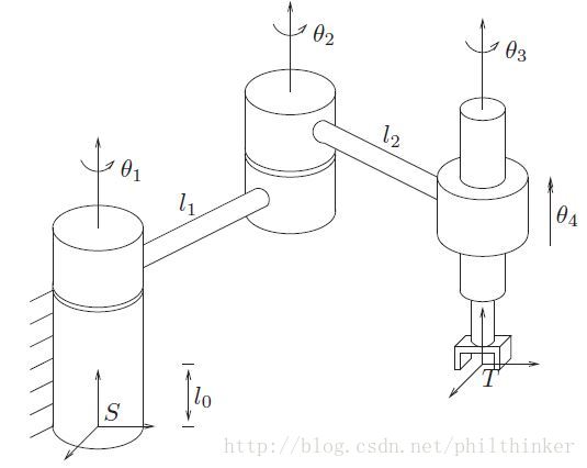
By inspection,

$$q_{1}'=\begin{bmatrix}0\\0\\0\end{bmatrix},\quad q_{1}'=\begin{bmatrix}-l_{1}s_{1}\\l_{1}c_{1}\\0\end{bmatrix}, \quad q_{1}'=\begin{bmatrix}-l_{1}s_{1}-l_{2}s_{12}\\l_{1}c_{1}+l_{2}c_{12}\\0\end{bmatrix}$$ are points on the axes. Calculating the associated twists yields
$$J_{st}^{s}=\begin{bmatrix} 0 & l_{1}c_{1} & l_{1}c_{1}+l_{2}c_{12} & 0 \\ 0 & l_{1}s_{1} & l_{1}s_{1}+l_{2}s_{12} & 0 \\ 0 & 0 & 0 & 1 \\ 0 & 0 & 0 & 0 \\ 0 & 0 & 0 & 0 \\ 1 & 1 & 1 & 0 \end{bmatrix}$$

The next section shows an alternative expression of Manipulator Jacobian.

Geometric Jacobian

Consider a n-link manipulator whose joint variables are $q_{1},\cdots, q_{n}$. Let

$$T^{0}_{n}=\begin{pmatrix}R^{0}_{n}(q) & o^{0}_{n}(q)\\0 & 1 \end{pmatrix}$$ denote the transformation from the end-effector frame to the base frame, where $q=(q_{1},\dots, q_{n})^{T}$ is the vector of joint variables. As the robot moves about, both the joint variables $q_i$ and the end-effector position $o_0^{n}$ and orientation $R_0^n$ will be functions of time. The objective of this section is to relate the linear and angular velocity of the end-effector to the vector of joint velocities $\dot{q}(t)$.
Define
$$S(\omega^{0}_{n})=\dot{R}^{0}_{n}(R^{0}_{n})^{T},\quad v^{0}_{n}=\dot{o}^{0}_{n}$$
We would like to formulate the following equations:
$$\begin{gather}v^{0}_{n}=J_{v}\dot{q}\\\omega^{0}_{n}=J_{\omega}\dot{q}\end{gather}$$
where $J_{v}$ and $J_{\omega}$ are $3\times n$ matrices. In a compact form:
$$\xi=J\dot{q},\qquad \xi=\begin{pmatrix} v_{n}^{0} \\ \omega_{n}^{0} \end{pmatrix},\quad J=\begin{pmatrix} J_{v} \\ J_{\omega} \end{pmatrix}$$
$J$ is called the Jacobian matrix that is a $6\times n$ matrix. $n$ is the number of links.

Angular Velocity

We can determine the angular velocity of the end-effector relative to the base by expressing the angular velocity contributed by each joint in the orientation of the base frame and then summing these.
If joint $i$ is a rotational joint whose axis is $z_{i-1}$, $q_{i}=\theta_{i}$. Let $\omega^{i-1}_{i}$ stand for the angular velocity of joint $i$ and link $i$ w.r.t. frame $o_{i-1}x_{i-1}y_{i-1}z_{i-1}$, i.e.

$$\omega^{i-1}_{i}=\dot{q}_{i}z^{i-1}_{i-1}=\dot{q}_{i}k$$
where $k=(0,0,1)^{T}$.
The angular velocity of the end-effector w.r.t. the base $\omega^{0}_{n}$ can be calculate by:
$$\omega^{0}_{n}=\rho_{1}\dot{q}_{1}k+\rho_{2}\dot{q}_{2}R^{0}_{1}k+\cdots +\rho_{n}\dot{q}_{n}R^{0}_{n-1}k=\sum^{n}_{i=1}\rho_{i}\dot{q}_{i}z^{0}_{i-1}$$
When joint $i$ is a rotational joint, $\rho_{i}=1$, or $\rho_{i}=0$. Then
$$J_{\omega}=(\rho_{1}z_{0}\cdots\rho_{n}z_{n-1})$$
All the $z_{i}$ is based on frame $o_{0}x_{0}y_{0}z_{0}$.

Linear Velocity

By the chain rule:

$$\dot{o}^{0}_{n}=\sum^{n}_{i=1}\frac{\partial o^{0}_{n}}{\partial q_{i}}\dot{q}_{i}$$ .
It is straightforward to see that the $i$ column of $J_{v}$ is
$$J_{vi}=\frac{\partial o^{0}_{n}}{\partial q_{i}}$$
Let us discuss two different types of joints separately.

Translational Joints

$$\begin{gather}\dot{o}^{0}_{n}=\dot{d}_{i}R^{0}_{i-1}\begin{pmatrix}0\\0\\1\end{pmatrix}= \dot{d}_{i}z^{0}_{i-1}\\J_{vi}=z_{i-1}\end{gather}$$

Rotational Joints

$$\begin{gather}\omega=\dot{\theta}_{i}z_{i-1}\\r=o_{n}-o_{i-1}\\J_{vi}=z_{i-1}\times (o_{n}-o_{i-1})\end{gather}$$

Jacobian Matrix

$$\begin{gather} J_{v}=(J_{v1} \cdots J_{vn})\\ J_{vi}=\left\{ \begin{aligned} & z_{i-1}\times (o_{n}-o_{i-1}), &\text{ for rotational joint } i\\&z_{i-1}, & \text{ for translational joint } i\end{aligned} \right. \\J_{\omega}=(J_{\omega1} \cdots J_{\omega n}) \\J_{\omega i}=\left\{ \begin{aligned} & z_{i-1}, &\text{ for rotational joint } i\\&0 & \text{ for translational joint } i\end{aligned}\right.\end{gather}$$
To calculate the Jacobian matrix, what we need is no more than the 3rd and 4th column of $T$.

Ex: Consider the two-link planar manipulator

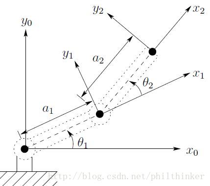
Since both joints are revolute the Jacobian matrix, which in this case is $6\times 2$, is of the form

$$J(q)=\begin{bmatrix} z_{0}\times (o_{2} - o_{0}) & z_{1}\times (o_{2}-o_{1}) \\ z_{0} & z_{1} \end{bmatrix}$$ The various quantities above are easily seen to be
$$o_{0}=\begin{bmatrix} 0 \\ 0 \\ 0 \end{bmatrix},\quad o_{1}=\begin{bmatrix} a_{1}c_{1} \\ a_{1}s_{1} \\ 0 \end{bmatrix},\quad o_{2}=\begin{bmatrix} a_{1}c_{1}+a_{2}c_{12} \\ a_{1}s_{1}+a_{2}s_{12} \\ 0 \end{bmatrix}$$
$$z_{0}=z_{1}=\begin{bmatrix} 0 \\ 0 \\ 1 \end{bmatrix}$$ Performing the required calculations then yields
$$J=\begin{bmatrix} -a_{1}s_{1}-a_{2}s_{12} & -a_{2}s_{12} \\ a_{1}c_{1}+a_{2}c_{12} & a_{2}c_{12} \\ 0 & 0 \\ 0 & 0 \\ 0 & 0\\ 1 & 1\end{bmatrix}$$

Changing a Jacobian’s Frame of Reference

Given a Jacobian written in frame $B$, that is

$$\begin{bmatrix}v^{B} \\ \omega^{B}\end{bmatrix}=J^{B}(\Theta)\dot{\Theta}$$ we might be interested in giving an expression for the Jacobian in another frame, $A$. Note:
$$\begin{bmatrix}v^{A} \\ \omega^{A}\end{bmatrix}=\begin{bmatrix}R_{B}^{A} & 0 \\ 0 & R_{B}^{A}\end{bmatrix} \begin{bmatrix}v^{B} \\ \omega^{B}\end{bmatrix}$$ Hence
$$J^{A}(\Theta)=\begin{bmatrix}R_{B}^{A} & 0 \\ 0 & R_{B}^{A}\end{bmatrix}J^{B}(\Theta)$$

Analytical Jacobian

Analytical Jacobian, $J_{a}(q)$, is the minimal representation of the end-effector.
Let

$$X=\begin{pmatrix}d(q)\\\alpha(q)\end{pmatrix}$$
stand for the configuration of the end-effector. $d(q)$ is the vector from the origin of the base frame to that of the end-effector. $\alpha=[\phi, \theta, \psi]^{T}$ is the Eular-Angular vector whose three partitions are called nutation, spin and precession.
We would like to find an equation of the following form:
$$\dot{X}\begin{pmatrix}\dot{d}\\\dot{\alpha}\end{pmatrix}=J_{a}(q)\dot{q}$$

If $R=R_{z,\phi}R_{y,\theta}R_{z,\psi}$ is an Eular Angular Transformation, it can proved that

$$\dot{R}=S(\omega)R$$
where the $\omega$, which defines the angular velocity, can be referred as:
$$\omega=\begin{pmatrix}c_{\psi}s_{\theta} & -s_{\psi} & 0\\s_{\psi}s_{\theta} & c_{\psi} & 0\\ c_{\theta} & 0 & 1\end{pmatrix}\begin{pmatrix}\dot{\phi}\\\dot{\theta}\\\dot{\psi}\end{pmatrix}=B(\alpha)\dot{\alpha}$$
Then
$$J(q)\dot{q}=\begin{pmatrix}v\\\omega\end{pmatrix}=\begin{pmatrix}\dot{d} \\ B(\alpha)\dot{\alpha} \end{pmatrix}=\begin{pmatrix}I & 0\\0 & B(\alpha)\end{pmatrix}\begin{pmatrix}\dot{d}\\\dot{\alpha}\end{pmatrix}=\begin{pmatrix}I & 0\\0 & B(\alpha)\end{pmatrix}J_{a}(q)\dot{q}$$
i.e.
$$J_{a}(q)=\begin{pmatrix}I & 0\\0 & B^{-1}(\alpha)\end{pmatrix}J(q)$$ once $\det B(\alpha)\neq 0$.

Singularities

A $6\times n$ Jacobian $J(q)$ defines a mapping from joint velocity $\dot{q}$ to end-effector velocity $\xi$, which also means that all the end-effector velocities can be represented by the linear combination of columns of Jacobian:

$$\xi=J_{1}\dot{q}_{1}+J_{2}\dot{q}_{2}+\cdots + J_{n}\dot{q}_{n}$$
For $\xi\in\mathbb{R}^{6}$, there must be 6 linear independent column vectors ( $\mathrm{rank} J=6$) so that the end-effector is able to perform any velocities.

It is straightforward to see that $\mathrm{rank}J\leq \min(6,n)$ for any $J\in\mathbb{R}^{6\times n}$. The rank of a Jacobian matrix depends on the configuration $q$. If the rank is less than its maximum value, the corresponding configuration is called singularity or singular configuration.

It is important to identify the singularities, since:

1. Singularities represent configurations from which certain directions of motion may be unattainable.
2. At singularities, bounded end-effector velocities may correspond to unbounded joint velocities.
3. At singularities, bounded end-effector forces and torques may correspond to unbounded joint torques.
4. Singularities usually (but not always) correspond to points on the boundary of the manipulator workspace, that is, to points of maximum reach of the manipulator.
5. Singularities correspond to points in the manipulator workspace that may be unreachable under small perturbations of the link parameters, such as length, offset, etc.
6. Near singularities there will not exist a unique solution to the inverse kinematics problem. In such cases there may be no solution or there may be infinitely many solutions.

All manipulators have singularities at the boundary of their workspace, and most have lots of singularities inside their workspace. We can class singularities into two categories:

1. Workspace-boundary singularities occur when the manipulator is fully stretched out or folded back on itself in such a way that the end-effector is at or very near the boundary of the workspace.
2. Workspace-inside singularities occur away from the boundary of workspace, and are usually generated from two or more collinear joint axes.

There are 3 common singularities for six degree of freedom manipulators:

1. Two collinear revolute joints: This type of singularity is common in spherical wrist assemblies that are composed of three mutually orthogonal revolute joints whose axes intersect at a point. In this configuration, rotation about the axis normal to the plane defined by the first and second joints is not possible.
2. Three parallel coplanar revolute joint axes: The Jacobian for a six degree of freedom manipulator is singular if there exist three revolute joints which satisfy the following conditions:(see also the figure below)
   
   1. The axes are parallel: $\omega_{i}=\pm\omega_{j}$ for $i,j=1,2,3$.
   2. The axes are coplanar : there exists a plane with unit normal $n$ such that $n^{T}\omega_{i}=0$ and $n^{T}(q_{i}-q_{j})=0, i,j=1,2,3$.
3. Four intersecting revolute joint axes: The Jacobian for a six degree of freedom manipulator is singular if there exist four revolute joint axes that intersect at a point $q$: $\omega_{i}\times(q_{i}-1)=0, i=1,\dots,4$.

It is also possible for a manipulator to exhibit different types of singularities at a single configuration. In this case, depending on the number and type of the singularities, the manipulator may lose the ability to move in several different directions at once.

Decoupling of Singularities

We can decouple the determination of singular configurations, for those manipulators with spherical wrists, into two simpler problems. The first is to determine so-called arm singularities, that is, singularities resulting from motion of the arm, which consists of the first three or more links, while the second is to determine the wrist singularities resulting from motion of the spherical wrist.

Suppose that $n=6$, that is, the manipulator consists of a $3$-DOF arm with a $3$-DOF spherical wrist. In this case the Jacobian is a $6\times 6$ matrix and a configuration q is singular if and only if

$$\det J(q)=0$$ If we now partition the Jacobian $J$ into $3\times 3$ blocks as
$$J=\begin{bmatrix}J_{P} & J_{O}\end{bmatrix}=\begin{bmatrix} J_{11} & J_{12} \\ J_{21} & J_{22} \end{bmatrix}$$ then, since the final three joints are always revolute
$$J_{O} = \begin{bmatrix} z_{3}\times(o_{6}-o_{3}) & z_{4}\times(o_{6}-o_{4}) & z_{5}\times(o_{6}-o_{5}) \\ z_{3} & z_{4} & z_{5} \end{bmatrix}$$ If we choose the coordinate frames so that $o_3 = o_4 = o_5 = o_6 = o$ (spherical wrist), then $J_{12}=0$. Furthermore,
$$\det J = \det J_{11}\det J_{22}$$ $J_{11}$ has $i$-th column $z_{i-1}\times(o-o_{i-1})$ if joint $i$ is revolute, and $z_{i-1}$ if joint $i$ is prismatic, while $J_{22}=[z_{3}, z_{4}, z_{5}]$. Note that this form of the Jacobian does not necessarily give the correct relation between the velocity of the end-effector and the joint velocities.