Systems biology informed deep learning for inferring parameters and hidden dynamics

作者：Alireza Yazdani1, Lu Lu1, Maziar Raissi2, George Em Karniadakis1
单位：

Division of Applied Mathematics, Brown University, Providence, RI 02912, USA,
Department of Applied Mathematics, University of Colorado, Boulder, CO 80309, USA

1 动机：

在系统集生物反应的数学模型可由带未知参数的ODE描述，使用reliable and robust的算法进行参数推断以及解的预测是系统生物学中的关键核心

2 主要研究内容：

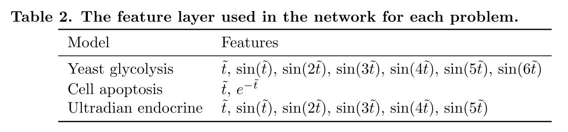
提出a new systems-biology-informed deep learning algorithm，该算法能够融合ODE到神经网络中
使用少量分散和噪声测量，能够对未观察的species、外部的动力学以及未知模型参数的dynamics进行推断
在三种不同的benchmark问题上进行测试

3 问题与方法

3.1 问题定义

$KaTeX parse error: {equation} can be used only in display mode.$ (1)
其中， $\mathbf{x}=\left(x_{1}, x_{2}, \ldots, x_{S}\right)$ 是 $S$ ， $\mathbf{p}=\left(p_{1}, p_{2}, \ldots, p_{K}\right)$ 是模型的 $K$ 个参数，需要被估计。一旦 $p$ 确定，该系统的ODE就能确定。 $\mathbf{y}$ 是 $M$ 个测量信号（带有高斯噪音的数据）。 $\mathbf{h}$ 由实验设计确定，可以为any function，在这假设为线性函数
$\left(\begin{array}{c} y_{1} \\ y_{2} \\ \cdots \\ y_{M} \end{array}\right)=\left(\begin{array}{c} x_{s_{1}} \\ x_{s_{2}} \\ \cdots \\ x_{s_{M}} \end{array}\right)+\left(\begin{array}{c} \epsilon_{s_{1}} \\ \epsilon_{s_{2}} \\ \cdots \\ \epsilon_{s_{M}} \end{array}\right)$ （2）

3.2 Systems-informed neural networks and parameter inference

![image.png](https://img-blog.csdnimg.cn/img_convert/eadcfac9abb0b3c4c3e6589ed0731c2b.png#align=left&display=inline&height=379&margin=[object Object]&name=image.png&originHeight=758&originWidth=1523&size=222031&status=done&style=none&width=761.5)
$KaTeX parse error: {equation} can be used only in display mode.$ （3）
$\mathcal{L}^{d a t a}(\boldsymbol{\theta})=\sum_{m=1}^{M} w_{m}^{d a t a} \mathcal{L}_{m}^{d a t a}=\sum_{m=1}^{M} w_{m}^{d a t a}\left[\frac{1}{N^{d a t a}} \sum_{n=1}^{N^{d a t a}}\left(y_{m}\left(t_{n}\right)-\hat{x}_{s_{m}}\left(t_{n} ; \boldsymbol{\theta}\right)\right)^{2}\right]$ （4）
$\mathcal{L}^{o d e}(\boldsymbol{\theta}, \mathbf{p})=\sum_{s=1}^{S} w_{s}^{o d e} \mathcal{L}_{s}^{o d e}=\sum_{s=1}^{S} w_{s}^{o d e}\left[\frac{1}{N^{o d e}} \sum_{n=1}^{N^{o d e}}\left(\left.\frac{d \hat{x}_{s}}{d t}\right|_{\tau_{n}}-f_{s}\left(\hat{x}_{s}\left(\tau_{n} ; \boldsymbol{\theta}\right), \tau_{n} ; \mathbf{p}\right)\right)^{2}\right]$ （5）
$\mathcal{L}^{a u x}(\boldsymbol{\theta})=\sum_{s=1}^{S} w_{s}^{a u x} \mathcal{L}_{s}^{a u x}=\sum_{s=1}^{S} w_{s}^{a u x} \frac{\left(x_{s}\left(T_{0}\right)-\hat{x}_{s}\left(T_{0} ; \boldsymbol{\theta}\right)\right)^{2}+\left(x_{s}\left(T_{1}\right)-\hat{x}_{s}\left(T_{1} ; \boldsymbol{\theta}\right)\right)^{2}}{2}$ （6）
前两项为data loss、ODE loss，最后一项为auxiliary loss，是系统的额外信息，包含两个时间点 $T_{0}$ 和 $T_{1}$ ，第一项与第三项属于监督loss，第二项为无监督loss。

在（4-6）中系数 $M + 2 S$ 个损失项，在这篇论文中，手动选择权重系数，使得加权的损失在网络训练中保持相同的数量级（待理解，为什么要一样数据集，是有什么特性吗）
对于第一项 $t_{1}, t_{2}, \ldots, t_{N^{d a t a}}$ ，随机采时间点；对于ODE loss中的time instant $\tau_{1}, \tau_{2}, \ldots, \tau_{N^{o d} e}$ 在一个等距离的网格中选择；第****三项 $T_{0}$ 为初值点， $T_{1}$ 可以在训练时间链上选择任意时间（但是不要离 $T_{0}$ 太近）

4 Analysis of system’s identifiability

在systems identification problems中，主要有两类identifiability，structural和practical。结构不可识别性由于 $y$ 解的冗余参数化，这是由于观测数据 $y$ 到 $x$ 的insufficient的映射 $\mathbf{h}$ 由于实验数据被忽视，出现了practical非识别性
结构上的可识别参数也可能是practical非识别性。practical非识别性与测量数据数量与质量有关，在一个无限的置信区间显示。

步骤

先考虑监督的loss(第一项和第三项)进行训练，使得网络能够快速拟合观察数据
然后再用三种损失进行训练

通过实验发现，这种两阶段训练策略加快了网络的收敛速度。

5 实验

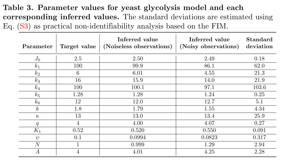
5.1 yeast glycolysis

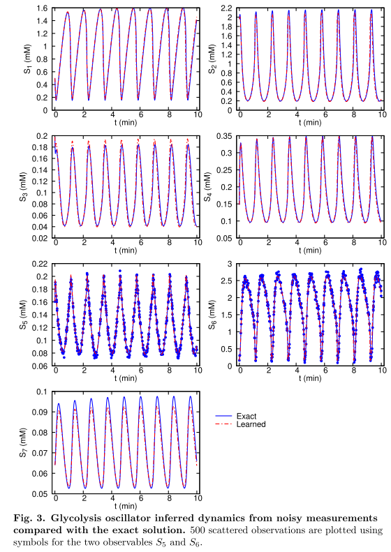
添加的ODE loss能防止网络过拟合
Standard deviation是基于FIM得到，结构/实际可识别性分析或bootstrapping方法获得参数置信区间，这里使用的是FIM

6 总结

利用网络训练拟合模型参数
提出了system-biology -informed 神经算法，能够可靠而准确的推断hidden dynamics
能够用很少的观测数据对dynamics和模型参数进行推断