MLflow 使用教程
- 本文翻译自 https://www.mlflow.org/docs/latest/concepts.html
- 本文地址 https://my.oschina.net/u/2306127/blog/1825690,by openthings, 2018.06.07.
参考:
- mlflow项目由Databricks创建。
- 基于Kubernetes的机器学习系统,https://my.oschina.net/u/2306127/blog/1822919
- Kubeflow-机器学习工作流框架,https://my.oschina.net/u/2306127/blog/1807785
- Spark机器学习工具链-MLflow,https://my.oschina.net/u/2306127/blog/1825638
What We’re Building
In this tutorial, we will showcase how a data scientist can use MLflow end to end to create a linear regression model; how we can use MLflow to package the code which trains this model in a reusable and reproducible model format; and finally how we can use MLflow to create a simple HTTP server which will enable us to score predictions.
For this tutorial we will use a dataset where we attempt to predict the quality of wine based on quantative features like the wine’s “fixed acidity”, “pH”, “residual sugar”, etc. The data-set we are using for this tutorial is from UCI’s machine learning repository. [Ref]
What You’ll Need
For this tutorial, we’ll be using MLflow, conda, and the tutorial code located at example/tutorial in the MLflow repository. To download the tutorial code run:
git clone https://github.com/databricks/mlflow
Training the Model
The first thing we’ll do is train a linear regression model which takes two hyperparameters: alpha and l1_ratio.
The code which we will use is located at example/tutorial/train.py and is reproduced below.
# Read the wine-quality csv file (make sure you're running this from the root of MLflow!)
wine_path = os.path.join(os.path.dirname(os.path.abspath(__file__)), "wine-quality.csv")
data = pd.read_csv(wine_path)

# Split the data into training and test sets. (0.75, 0.25) split.
train, test = train_test_split(data)

# The predicted column is "quality" which is a scalar from [3, 9]
train_x = train.drop(["quality"], axis=1)
test_x = test.drop(["quality"], axis=1)
train_y = train[["quality"]]
test_y = test[["quality"]]

alpha = float(sys.argv[1]) if len(sys.argv) > 1 else 0.5
l1_ratio = float(sys.argv[2]) if len(sys.argv) > 2 else 0.5

with mlflow.start_run():
    lr = ElasticNet(alpha=alpha, l1_ratio=l1_ratio, random_state=42)
    lr.fit(train_x, train_y)

    predicted_qualities = lr.predict(test_x)

    (rmse, mae, r2) = eval_metrics(test_y, predicted_qualities)

    print("Elasticnet model (alpha=%f, l1_ratio=%f):" % (alpha, l1_ratio))
    print("  RMSE: %s" % rmse)
    print("  MAE: %s" % mae)
    print("  R2: %s" % r2)

    mlflow.log_param("alpha", alpha)
    mlflow.log_param("l1_ratio", l1_ratio)
    mlflow.log_metric("rmse", rmse)
    mlflow.log_metric("r2", r2)
    mlflow.log_metric("mae", mae)

    mlflow.sklearn.log_model(lr, "model")
In this code, we use the familiar pandas, numpy, and sklearn APIs to create a simple machine learning model. In addition, we also use the MLflow tracking APIs to log information about each training run, like the hyperparameters alpha and l1_ratio we used to train the model and metrics like the root mean square error which we will use to evaluate the model. In addition, we serialize the model which we produced in a format that MLflow knows how to deploy.
To run this example execute:
python example/tutorial/train.py
Try out some other values for alpha and l1_ratio by passing them as arguments to train.py.:
python example/tutorial/train.py <alpha> <l1_ratio>
After running this, MLflow has logged information about your experiment runs in the directory called mlruns.
Comparing the Models
Next we will use the MLflow UI to compare the models which we have produced. Run mlflow ui in the same current working directory as the one which contains the mlruns directory and navigate your browser to http://localhost:5000.
On this page, we can see the metrics we can use to compare our models.
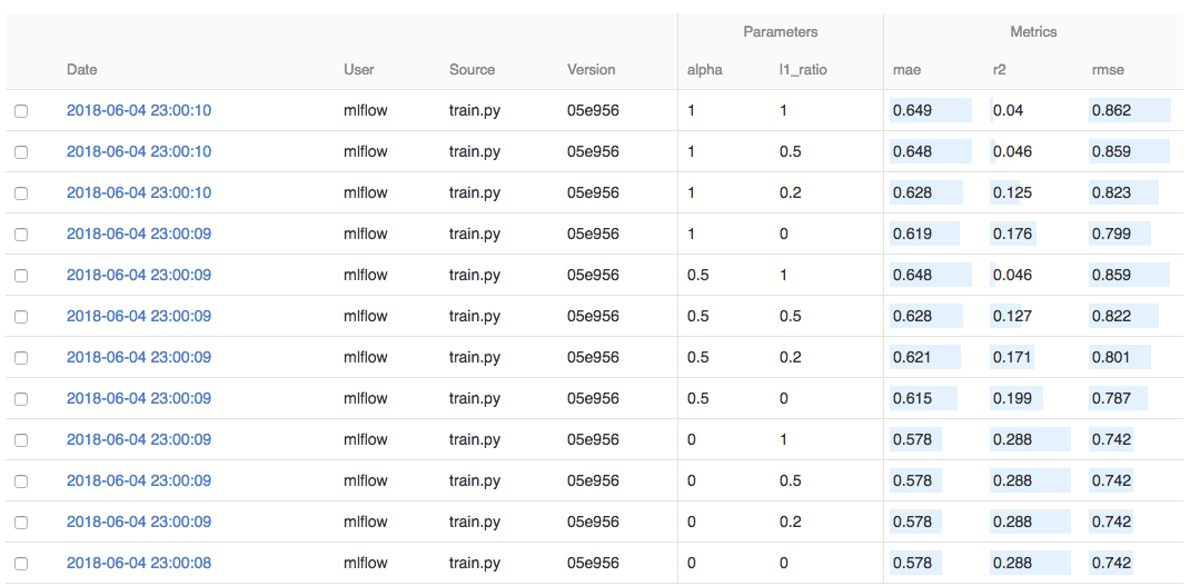
Using this page, we can see that the lower alpha is the better our model. We can also use the search feature to quickly filter out many models. For example the query metrics.rmse < 0.8 would return all the models with root mean squared error less than 0.8. For more complex manipulations, we can download this table as a CSV and use our favorite data munging software to analyze it.
Packaging the Training Code
Now that we have our training code written, we would like to package it so that other data scientists can easily reuse our model, or so that we can run the training remotely e.g. on Databricks. To do this, we use the MLflow Projects conventions to specify the dependencies and entry points to our code. In the example/tutorial/MLproject file we specify that our project has the dependencies located in the Conda environment file called conda.yaml and that our project has one entry point which takes two parameters: alpha and l1_ratio.
# example/tutorial/MLproject

name: tutorial

conda_env: conda.yaml

entry_points:
  main:
    parameters:
      alpha: float
      l1_ratio: {type: float, default: 0.1}
    command: "python train.py {alpha} {l1_ratio}"
# example/tutorial/conda.yaml

name: tutorial
channels:
  - defaults
dependencies:
  - numpy=1.14.3
  - pandas=0.22.0
  - scikit-learn=0.19.1
  - pip:
    - mlflow
To run this project, we simply invoke mlflow run example/tutorial -P alpha=0.42. After running this command, MLflow will run your training code in a new conda environment with the dependencies specified in conda.yaml.
Projects can also be run directly from Github if the repository has a MLproject file in the root. We’ve duplicated this tutorial to the https://github.com/databricks/mlflow-example repository which can be run with mlflow run [email protected]:databricks/mlflow-example.git -P alpha=0.42.
Serving the Model
Now that we have packaged our model using the MLproject convention and have identified the best model, it is time to deploy the model using MLflow Models. An MLflow Model is a standard format for packaging machine learning models that can be used in a variety of downstream tools — for example, real-time serving through a REST API or batch inference on Apache Spark.
In our example training code, after training the linear regression model, we invoked a function in MLflow which saved the model as an artifact within the run.
mlflow.sklearn.log_model(lr, "model")
To view this artifact, we can use the UI again. By clicking on a row in the listing of experiment runs we’ll see this page.
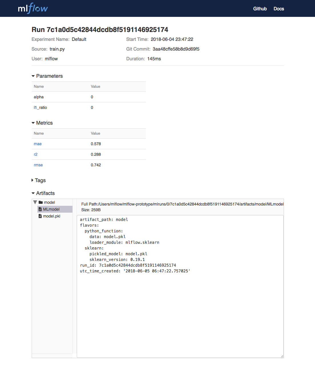
At the bottom, we can see that the call to mlflow.sklearn.log_model produced two files in/Users/mlflow/mlflow-prototype/mlruns/0/7c1a0d5c42844dcdb8f5191146925174/artifacts/model. The first file, MLmodel is a metadata file which tells MLflow how to load the model. The second file, model.pkl is a serialized version of the linear regression model which we trained.
In our example, we’ll demonstrate how we can use this MLmodel format with MLflow to deploy a local REST server which can serve predictions.
To deploy the server run:
mlflow sklearn serve /Users/mlflow/mlflow-prototype/mlruns/0/7c1a0d5c42844dcdb8f5191146925174/artifacts/model -p 1234
Note
The version of Python used to create the model must be the same as the one which is runningmlflow sklearn. If this is not the case, you may run into the errorUnicodeDecodeError: 'ascii' codec can't decode byte 0x9f in position 1: ordinal not in range(128) or raise ValueError, "unsupported pickle protocol: %d".
To serve a prediction run:
curl -X POST -H "Content-Type:application/json" --data '[{"fixed acidity": 6.2, "volatile acidity": 0.66, "citric acid": 0.48, "residual sugar": 1.2, "chlorides": 0.029, "free sulfur dioxide": 29, "total sulfur dioxide": 75, "density": 0.98, "pH": 3.33, "sulphates": 0.39, "alcohol": 12.8}]' http://127.0.0.1:1234/invocations

# RESPONSE
# {"predictions": [6.379428821398614]}
More Resources
Congratulations on finishing the tutorial! For more reading reference MLflow Tracking, MLflow Projects, MLflow Models, and more.