此文章为【我是土堆 - Pytorch教程】 知识点 学习总结笔记(四)包括:神经网络 - 非线性激活 、神经网络 - 线性层及其他层介绍 、神经网络 - 搭建小实战和 Sequential 的使用、损失函数与反向传播、优化器、现有网络模型的使用及修改、网络模型的保存与读取。
学习系列笔记(已完结):
【我是土堆 - Pytorch教程】 知识点 学习总结笔记(一)_耿鬼喝椰汁的博客-CSDN博客
【我是土堆 - Pytorch教程】 知识点 学习总结笔记(二)_耿鬼喝椰汁的博客-CSDN博客
【我是土堆 - Pytorch教程】 知识点 学习总结笔记(三)_耿鬼喝椰汁的博客-CSDN博客
【我是土堆 - Pytorch教程】 知识点 学习总结笔记(四)_耿鬼喝椰汁的博客-CSDN博客
【我是土堆 - Pytorch教程】 知识点 学习总结笔记(五)_耿鬼喝椰汁的博客-CSDN博客
目录
2.Recurrent Layers(特定网络中使用,自学)
3.Transformer Layers(特定网络中使用,自学)
4.Linear Layers--线性层(本节讲解)--使用较多
三、神经网络 - 搭建小实战和 Sequential 的使用
用 Sequential 搭建,实现上图 CIFAR10 model 的代码
3.如何在之前写的神经网络中用到 Loss Function(损失函数)
一、神经网络 - 非线性激活
使用到的pytorch网站:
-
Padding Layers(对输入图像进行填充的各种方式)
几乎用不到,nn.ZeroPad2d(在输入tensor数据类型周围用0填充)
nn.ConstantPad2d(用常数填充)
在 Conv2d 中可以实现,故不常用
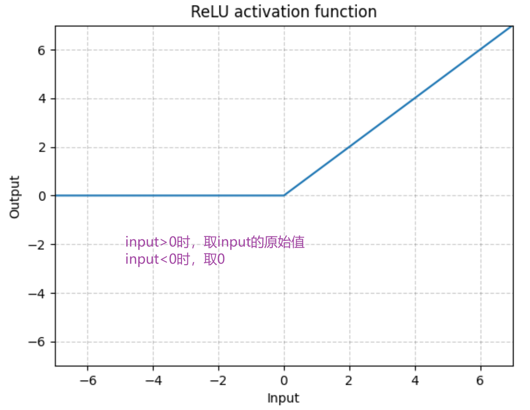
1.最常见的非线性激活:RELU
ReLU — PyTorch 1.10 documentation
输入:(N,*) N 为 batch_size,*不限制可以是任意
代码举例:RELU
import torch
from torch import nn
from torch.nn import ReLU

input = torch.tensor([[1,-0.5],
                      [-1,3]])
input = torch.reshape(input,(-1,1,2,2))  #input必须要指定batch_size,-1表示batch_size自己算,1表示是1维的
print(input.shape)   #torch.Size([1, 1, 2, 2])

# 搭建神经网络
class Tudui(nn.Module):
    def __init__(self):
        super(Tudui, self).__init__()
        self.relu1 = ReLU()  #inplace默认为False
    def forward(self,input):
        output = self.relu1(input)
        return output

# 创建网络
tudui = Tudui()
output = tudui(input)
print(output)
2.Sigmoid
Sigmoid — PyTorch 1.10 documentation


输入:(N,*) N 为 batch_size,*不限制
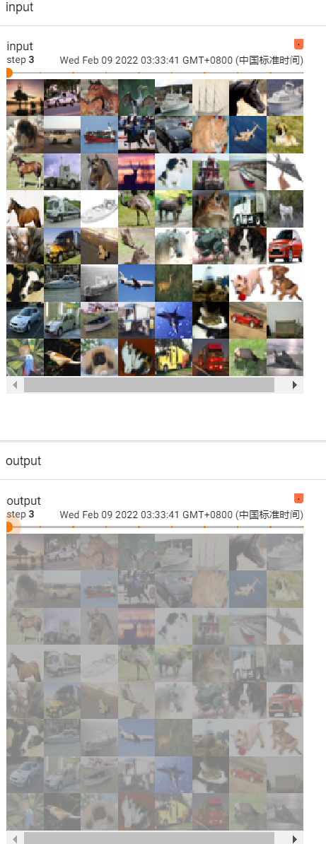
代码举例:Sigmoid(数据集CIFAR10)
import torch
import torchvision.datasets
from torch import nn
from torch.nn import Sigmoid
from torch.utils.data import DataLoader
from torch.utils.tensorboard import SummaryWriter

dataset = torchvision.datasets.CIFAR10("../data",train=False,download=True,transform=torchvision.transforms.ToTensor())
dataloader = DataLoader(dataset,batch_size=64)

# 搭建神经网络
class Tudui(nn.Module):
    def __init__(self):
        super(Tudui, self).__init__()
        self.sigmoid1 = Sigmoid()  #inplace默认为False
    def forward(self,input):
        output = self.sigmoid1(input)
        return output

# 创建网络
tudui = Tudui()

writer = SummaryWriter("../logs_sigmoid")
step = 0
for data in dataloader:
    imgs,targets = data
    writer.add_images("input",imgs,global_step=step)
    output = tudui(imgs)
    writer.add_images("output",output,step)
    step = step + 1

writer.close()
运行后在 terminal 里输入:
tensorboard --logdir=logs_sigmoid打开网址:
关于inplace

二.神经网络 - 线性层及其他层介绍
1.批标准化层--归一化层(不难,自学看官方文档)
torch.nn — PyTorch 1.10 documentation
BatchNorm2d — PyTorch 1.10 documentation
对输入采用Batch Normalization,可以加快神经网络的训练速度
CLASS torch.nn.BatchNorm2d(num_features, eps=1e-05, momentum=0.1, affine=True, track_running_stats=True, device=None, dtype=None)
# num_features C-输入的channel
# With Learnable Parameters
m = nn.BatchNorm2d(100)
# Without Learnable Parameters
m = nn.BatchNorm2d(100, affine=False) # 正则化层num_feature等于channel,即100
input = torch.randn(20, 100, 35, 45) #batch_size=20,100个channel,35x45的输入
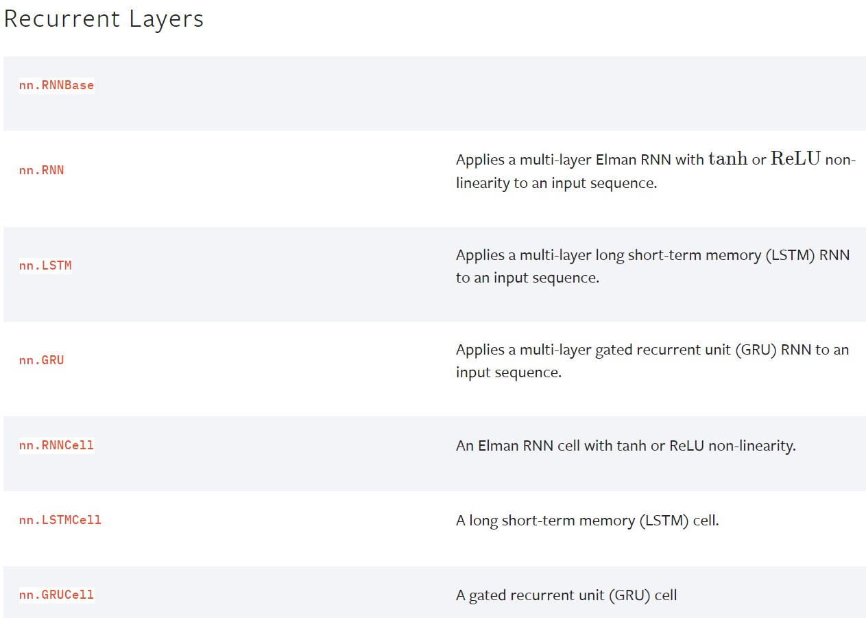
output = m(input)2.Recurrent Layers(特定网络中使用,自学)
RNN、LSTM等,用于文字识别中,特定的网络结构
torch.nn — PyTorch 1.13 documentation
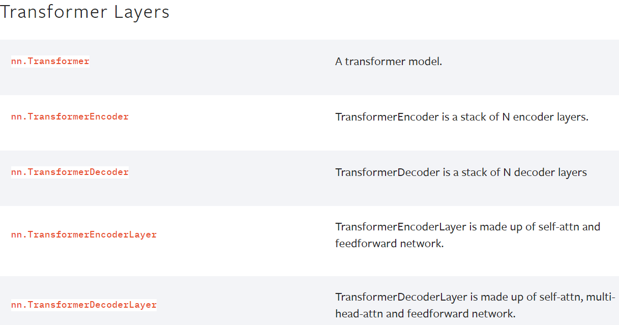
3.Transformer Layers(特定网络中使用,自学)
特定网络结构
torch.nn — PyTorch 1.13 documentation
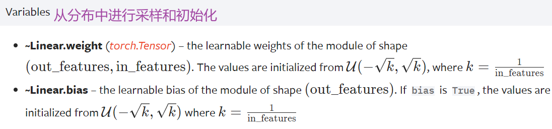
4.Linear Layers--线性层(本节讲解)--使用较多
网站地址:Linear — PyTorch 1.10 documentation

d代表特征数,L代表神经元个数 K和b在训练过程中神经网络会自行调整,以达到比较合理的预测

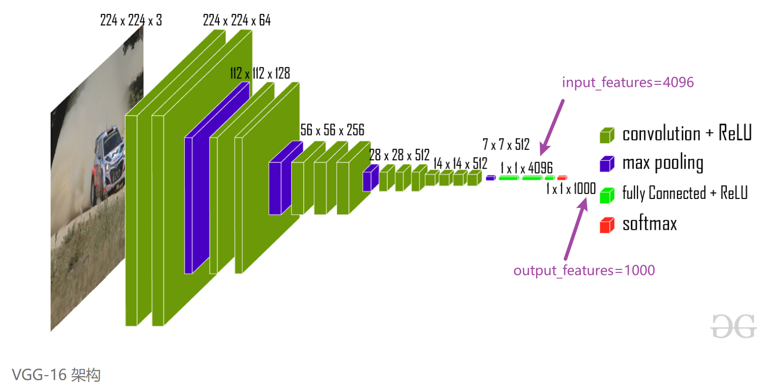
 5.代码实例 vgg16 model
flatten 摊平
torch.flatten — PyTorch 1.10 documentation
# Example
>>> t = torch.tensor([[[1, 2],
                   [3, 4]],
                  [[5, 6],
                   [7, 8]]])   #3个中括号,所以是3维的
>>> torch.flatten(t)  #摊平
tensor([1, 2, 3, 4, 5, 6, 7, 8])
>>> torch.flatten(t, start_dim=1)  #变为1行
tensor([[1, 2, 3, 4],
[5, 6, 7, 8]])- reshape():可以指定尺寸进行变换
- flatten():变成1行,摊平
output = torch.flatten(imgs)
# 等价于
output = torch.reshape(imgs,(1,1,1,-1))


for data in dataloader:
    imgs,targets = data
    print(imgs.shape)  #torch.Size([64, 3, 32, 32])
    output = torch.reshape(imgs,(1,1,1,-1))  # 想把图片展平
    print(output.shape)  # torch.Size([1, 1, 1, 196608])
    output = tudui(output)
    print(output.shape)  # torch.Size([1, 1, 1, 10])

for data in dataloader:
    imgs,targets = data
    print(imgs.shape)  #torch.Size([64, 3, 32, 32])
    output = torch.flatten(imgs)   #摊平
    print(output.shape)   #torch.Size([196608])
    output = tudui(output)
    print(output.shape)   #torch.Size([10])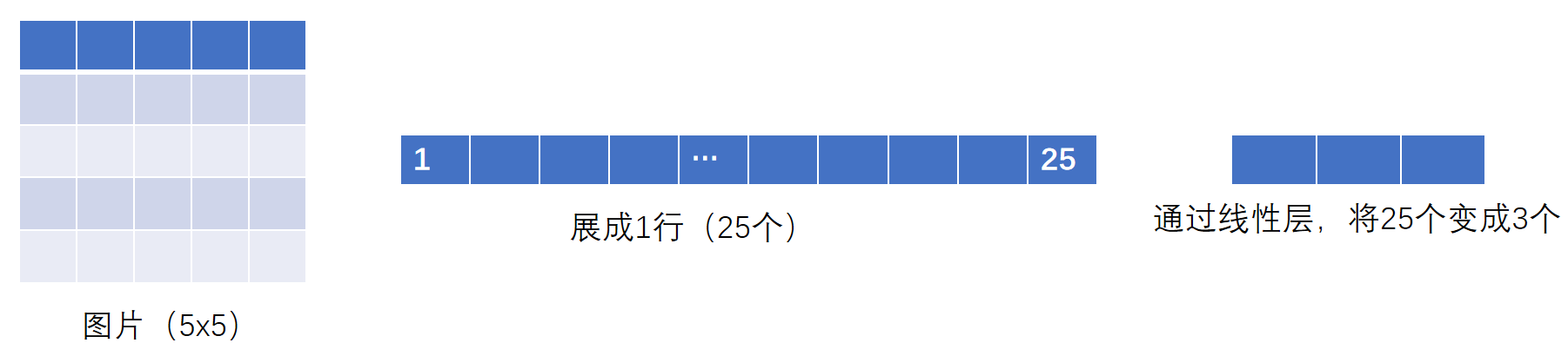
import torch
import torchvision.datasets
from torch import nn
from torch.nn import Linear
from torch.utils.data import DataLoader

dataset = torchvision.datasets.CIFAR10("../data",train=False,transform=torchvision.transforms.ToTensor(),download=True)
dataloader = DataLoader(dataset,batch_size=64,drop_last=True)

class Tudui(nn.Module):
    def __init__(self):
        super(Tudui, self).__init__()
        self.linear1 = Linear(196608,10)
    def forward(self,input):
        output = self.linear1(input)
        return output

tudui = Tudui()

for data in dataloader:
    imgs,targets = data
    print(imgs.shape)  #torch.Size([64, 3, 32, 32])
    # output = torch.reshape(imgs,(1,1,1,-1))  # 想把图片展平
    # print(output.shape)  # torch.Size([1, 1, 1, 196608])
    # output = tudui(output)
    # print(output.shape)  # torch.Size([1, 1, 1, 10])
    output = torch.flatten(imgs)   #摊平
    print(output.shape)   #torch.Size([196608])
    output = tudui(output)
    print(output.shape)   #torch.Size([10])
运行结果如下:

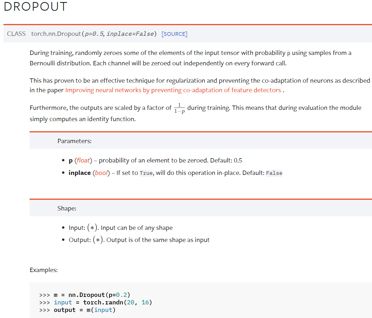
6.Dropout Layers(不难,自学)
Dropout — PyTorch 1.10 documentation
在训练过程中,随机把一些 input(输入的tensor数据类型)中的一些元素变为0,变为0的概率为p
目的:防止过拟合
7.Sparse Layers(特定网络中使用,自学)
Embedding
Embedding — PyTorch 1.10 documentation
用于自然语言处理
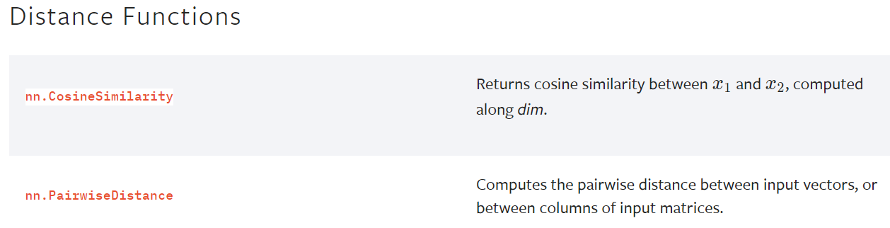
8.Distance Functions
计算两个值之间的误差
torch.nn — PyTorch 1.13 documentation
9. Loss Functions
loss 误差大小
torch.nn — PyTorch 1.13 documentation

10. pytorch提供的一些网络模型
- 图片相关:torchvision torchvision.models — Torchvision 0.11.0 documentation
分类、语义分割、目标检测、实例分割、人体关键节点识别(姿态估计)等等
- 文本相关:torchtext 无
- 语音相关:torchaudio torchaudio.models — Torchaudio 0.10.0 documentation
下一节:Container ——> Sequential(序列)
三、神经网络 - 搭建小实战和 Sequential 的使用
Containers中有Module、Sequential等
网站地址 : Sequential — PyTorch 1.10 documentation
Example:
# Using Sequential to create a small model. When `model` is run,
# input will first be passed to `Conv2d(1,20,5)`. The output of
# `Conv2d(1,20,5)` will be used as the input to the first
# `ReLU`; the output of the first `ReLU` will become the input
# for `Conv2d(20,64,5)`. Finally, the output of
# `Conv2d(20,64,5)` will be used as input to the second `ReLU`
model = nn.Sequential(
          nn.Conv2d(1,20,5),
          nn.ReLU(),
          nn.Conv2d(20,64,5),
          nn.ReLU()
        )

# Using Sequential with OrderedDict. This is functionally the
# same as the above code
model = nn.Sequential(OrderedDict([
          ('conv1', nn.Conv2d(1,20,5)),
          ('relu1', nn.ReLU()),
          ('conv2', nn.Conv2d(20,64,5)),
          ('relu2', nn.ReLU())
        ]))
好处:代码简洁易懂
1.对 CIFAR10 进行分类的简单神经网络
CIFAR 10:根据图片内容,识别其究竟属于哪一类(10代表有10个类别)
CIFAR-10 and CIFAR-100 datasets
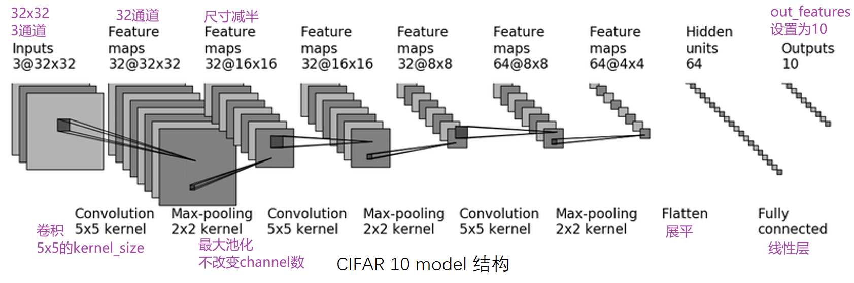
第一次卷积:首先加了几圈 padding(图像大小不变,还是32x32),然后卷积了32次
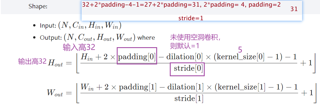
- Conv2d — PyTorch 1.10 documentation
- 输入尺寸是32x32,经过卷积后尺寸不变,如何设置参数? —— padding=2,stride=1
- 计算公式:
几个卷积核就是几通道的,一个卷积核作用于RGB三个通道后会把得到的三个矩阵的对应值相加,也就是说会合并,所以一个卷积核会产生一个通道
任何卷积核在设置padding的时候为保持输出尺寸不变都是卷积核大小的一半
通道变化时通过调整卷积核的个数(即输出通道)来实现的,在 nn.conv2d 的参数中有 out_channel 这个参数,就是对应输出通道
kernel 的内容是不一样的,可以理解为不同的特征抓取,因此一个核会产生一个channel
直接搭建,实现上图 CIFAR10 model 的代码
from torch import nn
from torch.nn import Conv2d, MaxPool2d, Flatten, Linear


class Tudui(nn.Module):
    def __init__(self):
        super(Tudui, self).__init__()
        self.conv1 = Conv2d(in_channels=3, out_channels=32, kernel_size=5, padding=2)  #第一个卷积
        self.maxpool1 = MaxPool2d(kernel_size=2)   #池化
        self.conv2 = Conv2d(32,32,5,padding=2)  #维持尺寸不变,所以padding仍为2
        self.maxpool2 = MaxPool2d(2)
        self.conv3 = Conv2d(32,64,5,padding=2)
        self.maxpool3 = MaxPool2d(2)
        self.flatten = Flatten()  #展平为64x4x4=1024个数据
        # 经过两个线性层:第一个线性层(1024为in_features,64为out_features)、第二个线性层(64为in_features,10为out_features)
        self.linear1 = Linear(1024,64)
        self.linear2 = Linear(64,10)  #10为10个类别,若预测的是概率,则取最大概率对应的类别,为该图片网络预测到的类别
    def forward(self,x):   #x为input
        x = self.conv1(x)
        x = self.maxpool1(x)
        x = self.conv2(x)
        x = self.maxpool2(x)
        x = self.conv3(x)
        x = self.maxpool3(x)
        x = self.flatten(x)
        x = self.linear1(x)
        x = self.linear2(x)
        return x

tudui = Tudui()
print(tudui)
可以看到网络结构:
实际过程中如何检查网络的正确性?
核心:一定尺寸的数据经过网络后,能够得到我们想要的输出
对网络结构进行检验的代码:
input = torch.ones((64,3,32,32))  #全是1,batch_size=64,3通道,32x32
output = tudui(input)
print(output.shape)
运行结果:
torch.Size([64, 10])若不知道flatten之后的维度是多少该怎么办?
from torch import nn
from torch.nn import Conv2d, MaxPool2d, Flatten, Linear


class Tudui(nn.Module):
    def __init__(self):
        super(Tudui, self).__init__()
        self.conv1 = Conv2d(in_channels=3, out_channels=32, kernel_size=5, padding=2)  #第一个卷积
        self.maxpool1 = MaxPool2d(kernel_size=2)   #池化
        self.conv2 = Conv2d(32,32,5,padding=2)  #维持尺寸不变,所以padding仍为2
        self.maxpool2 = MaxPool2d(2)
        self.conv3 = Conv2d(32,64,5,padding=2)
        self.maxpool3 = MaxPool2d(2)
        self.flatten = Flatten()  #展平为64x4x4=1024个数据
        # 经过两个线性层:第一个线性层(1024为in_features,64为out_features)、第二个线性层(64为in_features,10为out_features)
        self.linear1 = Linear(1024,64)
        self.linear2 = Linear(64,10)  #10为10个类别,若预测的是概率,则取最大概率对应的类别,为该图片网络预测到的类别
    def forward(self,x):   #x为input
        x = self.conv1(x)
        x = self.maxpool1(x)
        x = self.conv2(x)
        x = self.maxpool2(x)
        x = self.conv3(x)
        x = self.maxpool3(x)
        x = self.flatten(x)
        return x

tudui = Tudui()
print(tudui)

input = torch.ones((64,3,32,32))  #全是1,batch_size=64(64张图片),3通道,32x32
output = tudui(input)
print(output.shape)  # torch.Size([64,1024])
看到输出的维度是(64,1024),64可以理解为64张图片,1024就是flatten之后的维度了
运行结果: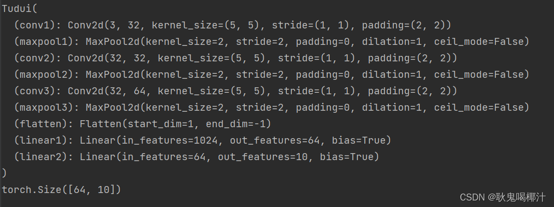
用 Sequential 搭建,实现上图 CIFAR10 model 的代码
作用:代码更加简洁
import torch
from torch import nn
from torch.nn import Conv2d, MaxPool2d, Flatten, Linear, Sequential


class Tudui(nn.Module):
    def __init__(self):
        super(Tudui, self).__init__()
        self.model1 = Sequential(
            Conv2d(3,32,5,padding=2),
            MaxPool2d(2),
            Conv2d(32,32,5,padding=2),
            MaxPool2d(2),
            Conv2d(32,64,5,padding=2),
            MaxPool2d(2),
            Flatten(),
            Linear(1024,64),
            Linear(64,10)
        )

    def forward(self,x):   #x为input
        x = self.model1(x)
        return x

tudui = Tudui()
print(tudui)

input = torch.ones((64,3,32,32))  #全是1,batch_size=64,3通道,32x32
output = tudui(input)
print(output.shape)
运行结果:

2.引入 tensorboard 可视化模型结构
在上述代码后面加上以下代码:
from torch.utils.tensorboard import SummaryWriter
writer = SummaryWriter("../logs_seq")
writer.add_graph(tudui,input)   # add_graph 计算图
writer.close()
运行后在 terminal 里输入:
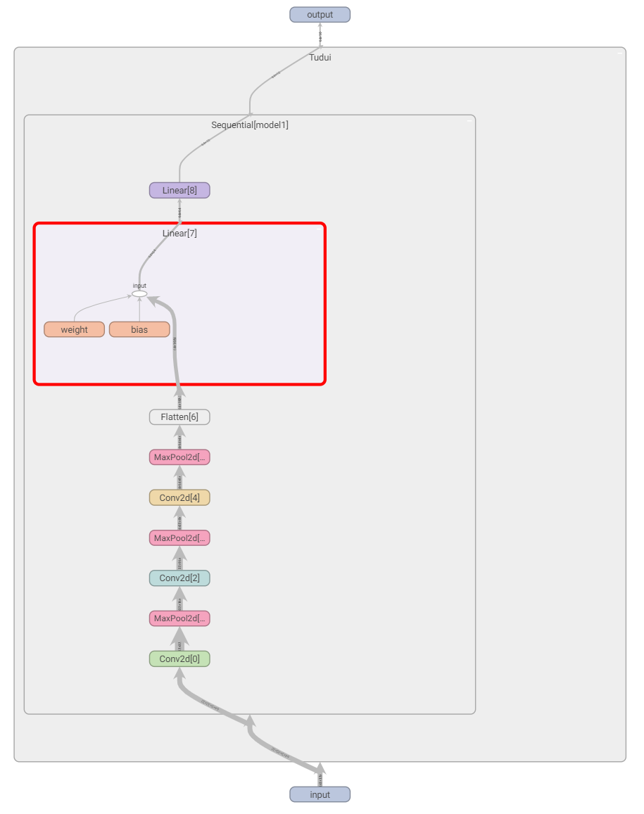
tensorboard --logdir=logs_seq打开网址,双击图片中的矩形,可以放大每个部分:
四、损失函数与反向传播
torch.nn 里的 loss function 衡量误差,在使用过程中根据需求使用,注意输入形状和输出形状即可
loss 衡量实际神经网络输出 output 与真实想要结果 target 的差距,越小越好
作用:
- 1. 计算实际输出和目标之间的差距
- 2. 为我们更新输出提供一定的依据(反向传播):给每一个卷积核中的参数提供了梯度 grad,采用反向传播时,每一个要更新的参数都会计算出对应的梯度,优化过程中根据梯度对参数进行优化,最终达到整个 loss 进行降低的目的
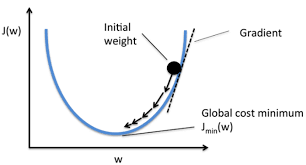
梯度下降法:
1. L1LOSS

input:(N,*) N是batch_size,即有多少个数据;*可以是任意维度
CLASS torch.nn.L1Loss(size_average=None, reduce=None, reduction='mean')小例子:
代码
import torch
from torch.nn import L1Loss
# 实际数据或网络默认情况下就是float类型,不写测试案例的话一般不需要加dtype
inputs = torch.tensor([1,2,3],dtype=torch.float32) # 计算时要求数据类型为浮点数,不能是整型的long
targets = torch.tensor([1,2,5],dtype=torch.float32)
inputs = torch.reshape(inputs,(1,1,1,3)) # 1 batch_size, 1 channel, 1行3列
targets = torch.reshape(targets,(1,1,1,3))
loss = L1Loss()
result = loss(inputs,targets)
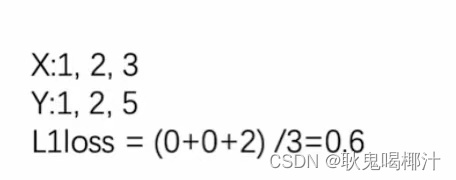
print(result)运行结果:
tensor(0.6667)求和的方式:
修改上述代码中的一句即可
loss = L1Loss(reduction='sum')运行结果:
tensor(2.)2.MSELOSS(均方误差)
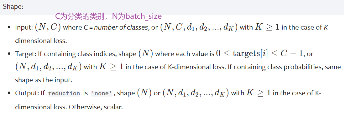
input:(N,*) N是batch_size,即有多少个数据;*可以是任意维度
CLASS torch.nn.MSELoss(size_average=None, reduce=None, reduction='mean')
代码:
import torch
from torch import nn
# 实际数据或网络默认情况下就是float类型,不写测试案例的话一般不需要加dtype
inputs = torch.tensor([1,2,3],dtype=torch.float32) # 计算时要求数据类型为浮点数,不能是整型的long
targets = torch.tensor([1,2,5],dtype=torch.float32)
inputs = torch.reshape(inputs,(1,1,1,3)) # 1 batch_size, 1 channel, 1行3列
targets = torch.reshape(targets,(1,1,1,3))
loss_mse = nn.MSELoss()
result_mse = loss_mse(inputs,targets)
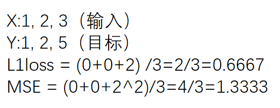
print(result_mse)结果:
![]()
上述代码的例子:
3. CROSSENTROPYLOSS(交叉熵)
适用于训练分类问题,有C个类别
例:三分类问题,person,dog,cat
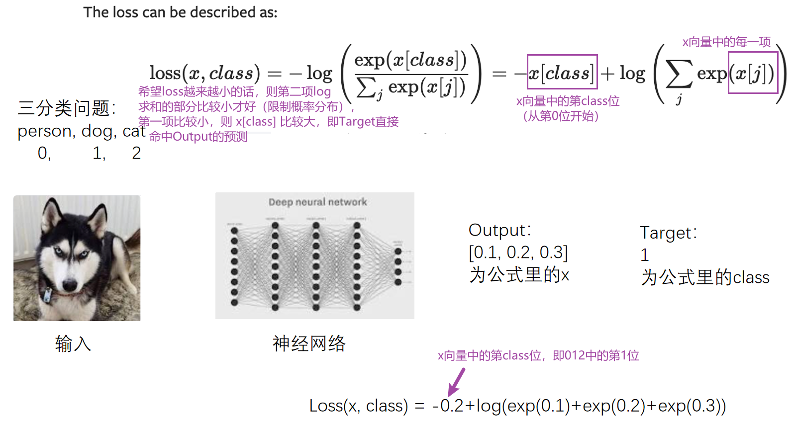
(公式中的 log 可以按 ln 算)
这里的output不是概率,是评估分数
代码:
x = torch.tensor([0.1,0.2,0.3])
y = torch.tensor([1])
x = torch.reshape(x,(1,3))
loss_cross = nn.CrossEntropyLoss()
result_cross = loss_cross(x,y)
print(result_cross)
结果:
tensor(1.1019)3.如何在之前写的神经网络中用到 Loss Function(损失函数)
import torchvision.datasets
from torch import nn
from torch.nn import Conv2d, MaxPool2d, Flatten, Linear, Sequential
from torch.utils.data import DataLoader

dataset = torchvision.datasets.CIFAR10("../data",train=False,transform=torchvision.transforms.ToTensor(),download=True)
dataloader = DataLoader(dataset,batch_size=1)

class Tudui(nn.Module):
    def __init__(self):
        super(Tudui, self).__init__()
        self.model1 = Sequential(
            Conv2d(3,32,5,padding=2),
            MaxPool2d(2),
            Conv2d(32,32,5,padding=2),
            MaxPool2d(2),
            Conv2d(32,64,5,padding=2),
            MaxPool2d(2),
            Flatten(),
            Linear(1024,64),
            Linear(64,10)
        )

    def forward(self,x):   # x为input
        x = self.model1(x)
        return x

loss = nn.CrossEntropyLoss()

tudui = Tudui()

for data in dataloader:
    imgs,targets = data  # imgs为输入,放入神经网络中
    outputs = tudui(imgs)  # outputs为输入通过神经网络得到的输出,targets为实际输出
    result_loss = loss(outputs,targets)
    print(result_loss)  # 神经网络输出与真实输出的误差
结果:

5. backward 反向传播
计算出每一个节点参数的梯度
在上述代码后加一行:
result_loss.backward() # backward反向传播,是对result_loss,而不是对loss在这一句代码前打上断点(运行到该行代码的前一行,该行不运行),debug 后:
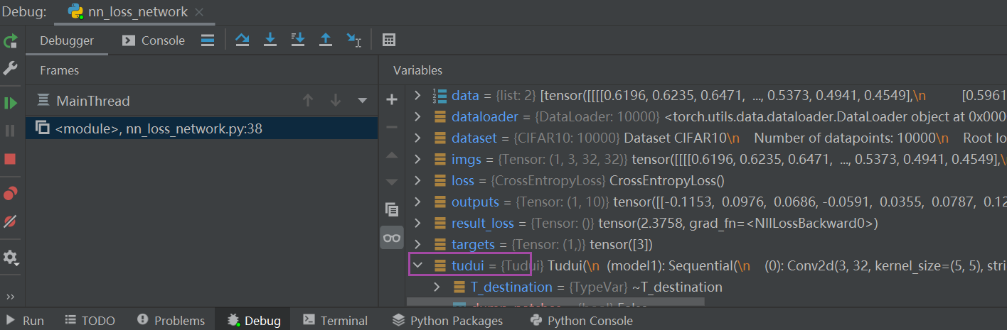
tudui ——> model 1 ——> Protected Attributes ——> _modules ——> '0' ——> bias / weight——> grad(是None)
点击Step into My Code,运行完该行后,可以发现刚刚的None有值了(损失函数一定要经过 .backward() 后才能反向传播,才能有每个需要调节的参数的grad的值)
下一节:选择合适的优化器,利用梯度对网络中的参数进行优化更新,以达到整个 loss最低的目的
五、优化器
当使用损失函数时,可以调用损失函数的 backward,得到反向传播,反向传播可以求出每个需要调节的参数对应的梯度,有了梯度就可以利用优化器,优化器根据梯度对参数进行调整,以达到整体误差降低的目的。
网站 : torch.optim — PyTorch 1.10 documentation
1.如何使用优化器?
(1)构造
# Example:
# SGD为构造优化器的算法,Stochastic Gradient Descent 随机梯度下降
optimizer = optim.SGD(model.parameters(), lr=0.01, momentum=0.9)  #模型参数、学习速率、特定优化器算法中需要设定的参数
optimizer = optim.Adam([var1, var2], lr=0.0001)
(2)调用优化器的step方法
利用之前得到的梯度对参数进行更新
for input, target in dataset:
    optimizer.zero_grad() #把上一步训练的每个参数的梯度清零
    output = model(input)
    loss = loss_fn(output, target)  # 输出跟真实的target计算loss
    loss.backward() #调用反向传播得到每个要更新参数的梯度
    optimizer.step() #每个参数根据上一步得到的梯度进行优化
算法
如Adadelta、Adagrad、Adam、RMSProp、SGD等等,不同算法前两个参数:params、lr 都是一致的,后面的参数不同
CLASS torch.optim.Adadelta(params, lr=1.0, rho=0.9, eps=1e-06, weight_decay=0)
# params为模型的参数、lr为学习速率(learning rate)
# 后续参数都是特定算法中需要设置的
学习速率不能太大(太大模型训练不稳定)也不能太小(太小模型训练慢),一般建议先采用较大学习速率,后采用较小学习速率
SGD为例
以 SGD(随机梯度下降法)为例进行说明:
import torch
import torchvision.datasets
from torch import nn
from torch.nn import Conv2d, MaxPool2d, Flatten, Linear, Sequential
from torch.utils.data import DataLoader

# 加载数据集并转为tensor数据类型
dataset = torchvision.datasets.CIFAR10("../data",train=False,transform=torchvision.transforms.ToTensor(),download=True)
# 加载数据集
dataloader = DataLoader(dataset,batch_size=1)

# 创建网络名叫Tudui
class Tudui(nn.Module):
    def __init__(self):
        super(Tudui, self).__init__()
        self.model1 = Sequential(
            Conv2d(3,32,5,padding=2),
            MaxPool2d(2),
            Conv2d(32,32,5,padding=2),
            MaxPool2d(2),
            Conv2d(32,64,5,padding=2),
            MaxPool2d(2),
            Flatten(),
            Linear(1024,64),
            Linear(64,10)
        )

    def forward(self,x):   # x为input,forward前向传播
        x = self.model1(x)
        return x

# 计算loss
loss = nn.CrossEntropyLoss()

# 搭建网络
tudui = Tudui()

# 设置优化器
optim = torch.optim.SGD(tudui.parameters(),lr=0.01)  # SGD随机梯度下降法

for data in dataloader:
    imgs,targets = data  # imgs为输入,放入神经网络中
    outputs = tudui(imgs)  # outputs为输入通过神经网络得到的输出,targets为实际输出
    result_loss = loss(outputs,targets)
    optim.zero_grad()  # 把网络模型中每一个可以调节的参数对应梯度设置为0
    result_loss.backward()  # backward反向传播求出每一个节点的梯度,是对result_loss,而不是对loss
    optim.step()  # 对每个参数进行调优
可以在以下地方打断点,debug:

tudui ——> Protected Attributes ——> _modules ——> 'model1' ——> Protected Attributes ——> _modules ——> '0' ——> weight ——> data 或 grad
通过每次按箭头所指的按钮(点一次运行一行),观察 data 和 grad 值的变化
- 第一行 optim.zero_grad() 是让grad清零
- 第三行 optim.step() 会通过grad更新data

完整代码
在 data 循环外又套一层 epoch 循环,一次 data 循环相当于对数据训练一次,加了 epoch 循环相当于对数据训练 20 次
import torch
import torchvision.datasets
from torch import nn
from torch.nn import Conv2d, MaxPool2d, Flatten, Linear, Sequential
from torch.utils.data import DataLoader

# 加载数据集并转为tensor数据类型
dataset = torchvision.datasets.CIFAR10("../data",train=False,transform=torchvision.transforms.ToTensor(),download=True)
dataloader = DataLoader(dataset,batch_size=1)

# 创建网络名叫Tudui
class Tudui(nn.Module):
    def __init__(self):
        super(Tudui, self).__init__()
        self.model1 = Sequential(
            Conv2d(3,32,5,padding=2),
            MaxPool2d(2),
            Conv2d(32,32,5,padding=2),
            MaxPool2d(2),
            Conv2d(32,64,5,padding=2),
            MaxPool2d(2),
            Flatten(),
            Linear(1024,64),
            Linear(64,10)
        )

    def forward(self,x):   # x为input,forward前向传播
        x = self.model1(x)
        return x

# 计算loss
loss = nn.CrossEntropyLoss()

# 搭建网络
tudui = Tudui()

# 设置优化器
optim = torch.optim.SGD(tudui.parameters(),lr=0.01)  # SGD随机梯度下降法
for epoch in range(20):
    running_loss = 0.0  # 在每一轮开始前将loss设置为0
    for data in dataloader:  # 该循环相当于只对数据进行了一轮学习
        imgs,targets = data  # imgs为输入,放入神经网络中
        outputs = tudui(imgs)  # outputs为输入通过神经网络得到的输出,targets为实际输出
        result_loss = loss(outputs,targets)
        optim.zero_grad()  # 把网络模型中每一个可以调节的参数对应梯度设置为0
        result_loss.backward()  # backward反向传播求出每一个节点的梯度,是对result_loss,而不是对loss
        optim.step()  # 对每个参数进行调优
        running_loss = running_loss + result_loss  # 每一轮所有loss的和
    print(running_loss)
部分运行结果:
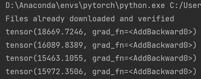
优化器对模型参数不断进行优化,每一轮的 loss 在不断减小
实际过程中模型在整个数据集上的训练次数(即最外层的循环)都是成百上千/万的,本例仅以 20 次为例。
六、现有网络模型的使用及修改

本节主要讲解 torchvision

本节主要讲解 Classification 里的 VGG 模型,数据集仍为 CIFAR10 数据集(主要用于分类)
网站 : torchvision.models — Torchvision 0.11.0 documentation
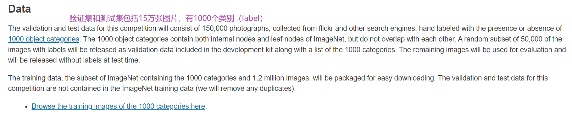
1.数据集 ImageNet
注意:必须要先有 package scipy
在 Terminal 里输入
pip list寻找是否有 scipy,若没有的话输入
pip install scipy(注意关闭代理)
参数及下载
1.参数:

2.下载 ImageNet 数据集:
import torchvision.datasets
train_data = torchvision.datasets.ImageNet("../data_image_net",split='train',download=True,
                                           transform=torchvision.transforms.ToTensor())
./xxx表示当前路径下,../xxx表示返回上一级目录
多行注释快捷键:ctrl+/
运行后会报错:
RuntimeError: The dataset is no longer publicly accessible. You need to download the archives externally and place them in the root directory.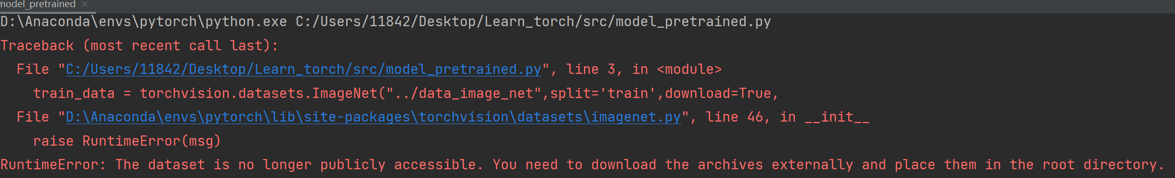
下载地址:
Imagenet 完整数据集下载_wendell 的博客-CSDN博客_imagenet下载
100 多个G,太大... 放弃
按住 Ctrl 键,点击 ImageNet,查看其源码:

2.VGG16 模型
VGG 11/13/16/19 常用16和19
(1)参数
参数 pretrained=True/False
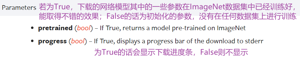
- pretrained 为 False 的情况下,只是加载网络模型,参数都为默认参数,不需要下载
- 为 True 时需要从网络中下载,卷积层、池化层对应的参数等等(在ImageNet数据集中训练好的)
import torchvision.models

vgg16_false = torchvision.models.vgg16(pretrained=False)  # 另一个参数progress显示进度条,默认为True
vgg16_true = torchvision.models.vgg16(pretrained=True)
print('ok')
断点打在 print('ok') 前,debug 一下,结果如图:

vgg16_true ——> classifier ——> Protected Attributes ——> modules ——> '0'(线性层) ——> weight

为 false 的情况,同理找到 weight 值:

总结:
- 设置为 False 的情况,相当于网络模型中的参数都是初始化的、默认的
- 设置为 True 时,网络模型中的参数在数据集上是训练好的,能达到比较好的效果
(2)vgg16 网络架构
import torchvision.models

vgg16_false = torchvision.models.vgg16(pretrained=False)  # 另一个参数progress显示进度条,默认为True
vgg16_true = torchvision.models.vgg16(pretrained=True)

print(vgg16_true)
输出:
VGG(
  (features): Sequential(
# 输入图片先经过卷积,输入是3通道的、输出是64通道的,卷积核大小是3×3的
    (0): Conv2d(3, 64, kernel_size=(3, 3), stride=(1, 1), padding=(1, 1))
# 非线性
    (1): ReLU(inplace=True)
# 卷积、非线性、池化...
    (2): Conv2d(64, 64, kernel_size=(3, 3), stride=(1, 1), padding=(1, 1))
    (3): ReLU(inplace=True)
    (4): MaxPool2d(kernel_size=2, stride=2, padding=0, dilation=1, ceil_mode=False)
    (5): Conv2d(64, 128, kernel_size=(3, 3), stride=(1, 1), padding=(1, 1))
    (6): ReLU(inplace=True)
    (7): Conv2d(128, 128, kernel_size=(3, 3), stride=(1, 1), padding=(1, 1))
    (8): ReLU(inplace=True)
    (9): MaxPool2d(kernel_size=2, stride=2, padding=0, dilation=1, ceil_mode=False)
    (10): Conv2d(128, 256, kernel_size=(3, 3), stride=(1, 1), padding=(1, 1))
    (11): ReLU(inplace=True)
    (12): Conv2d(256, 256, kernel_size=(3, 3), stride=(1, 1), padding=(1, 1))
    (13): ReLU(inplace=True)
    (14): Conv2d(256, 256, kernel_size=(3, 3), stride=(1, 1), padding=(1, 1))
    (15): ReLU(inplace=True)
    (16): MaxPool2d(kernel_size=2, stride=2, padding=0, dilation=1, ceil_mode=False)
    (17): Conv2d(256, 512, kernel_size=(3, 3), stride=(1, 1), padding=(1, 1))
    (18): ReLU(inplace=True)
    (19): Conv2d(512, 512, kernel_size=(3, 3), stride=(1, 1), padding=(1, 1))
    (20): ReLU(inplace=True)
    (21): Conv2d(512, 512, kernel_size=(3, 3), stride=(1, 1), padding=(1, 1))
    (22): ReLU(inplace=True)
    (23): MaxPool2d(kernel_size=2, stride=2, padding=0, dilation=1, ceil_mode=False)
    (24): Conv2d(512, 512, kernel_size=(3, 3), stride=(1, 1), padding=(1, 1))
    (25): ReLU(inplace=True)
    (26): Conv2d(512, 512, kernel_size=(3, 3), stride=(1, 1), padding=(1, 1))
    (27): ReLU(inplace=True)
    (28): Conv2d(512, 512, kernel_size=(3, 3), stride=(1, 1), padding=(1, 1))
    (29): ReLU(inplace=True)
    (30): MaxPool2d(kernel_size=2, stride=2, padding=0, dilation=1, ceil_mode=False)
  )
  (avgpool): AdaptiveAvgPool2d(output_size=(7, 7))
  (classifier): Sequential(
    (0): Linear(in_features=25088, out_features=4096, bias=True)
    (1): ReLU(inplace=True)
    (2): Dropout(p=0.5, inplace=False)
    (3): Linear(in_features=4096, out_features=4096, bias=True)
    (4): ReLU(inplace=True)
    (5): Dropout(p=0.5, inplace=False)
# 最后线性层输出为1000(vgg16也是一个分类模型,能分出1000个类别)
    (6): Linear(in_features=4096, out_features=1000, bias=True)
  )
)
所以 out_features = 1000
3.如何利用现有网络去改动它的结构?
train_data = torchvision.datasets.CIFAR10(root="./dataset",train=True,transform=torchvision.transforms.ToTensor(),download=True)CIFAR10 把数据分成了10类,而 vgg16 模型把数据分成了 1000 类,如何应用这个网络模型呢?
- 1. 把最后线性层的 out_features 从1000改为10
- 2. 在最后的线性层下面再加一层,in_features为1000,out_features为10
利用现有网络去改动它的结构,避免写 vgg16
很多框架会把 vgg16 当做前置的网络结构,提取一些特殊的特征,再在后面加一些网络结构,实现功能。
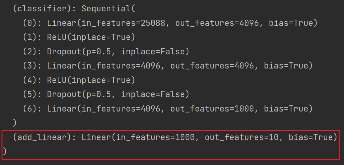
(1)添加
以 vgg16_true 为例讲解,实现上面的第二种思路:
# 给 vgg16 添加一个线性层,输入1000个类别,输出10个类别
vgg16_true.add_module('add_linear',nn.Linear(in_features=1000,out_features=10))
print(vgg16_true)
结果如图:
如果想将 module 添加至 classifier 里:
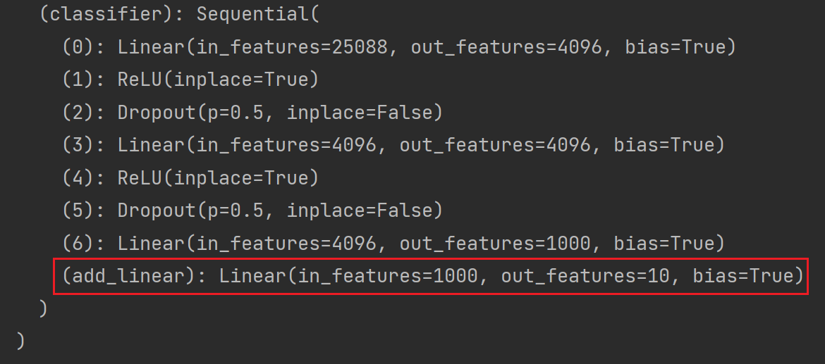
# 给 vgg16 添加一个线性层,输入1000个类别,输出10个类别
vgg16_true.classifier.add_module('add_linear',nn.Linear(in_features=1000,out_features=10))
print(vgg16_true)
结果如图:
(2)修改
以上为添加,那么如何修改呢?
以 vgg16_false 为例:
vgg16_false = torchvision.models.vgg16(pretrained=False)  # 另一个参数progress显示进度条,默认为True
print(vgg16_false)
结果如下:
(classifier): Sequential(
(0): Linear(in_features=25088, out_features=4096, bias=True)
(1): ReLU(inplace=True)
(2): Dropout(p=0.5, inplace=False)
(3): Linear(in_features=4096, out_features=4096, bias=True)
(4): ReLU(inplace=True)
(5): Dropout(p=0.5, inplace=False)
(6): Linear(in_features=4096, out_features=1000, bias=True)
)
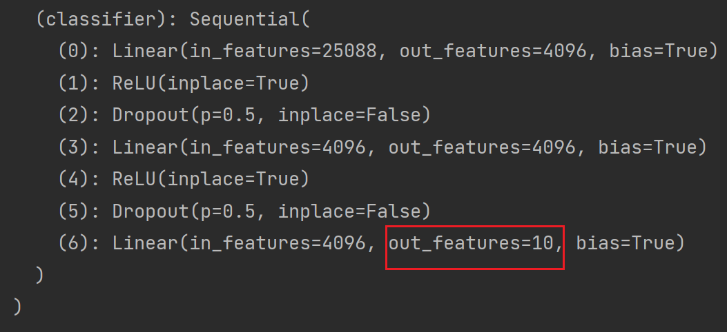
)想将最后一层 Linear 的 out_features 改为10:
vgg16_false.classifier[6] = nn.Linear(4096,10)
print(vgg16_false)
结果如下:
本节:
- 如何加载现有的一些 pytorch 提供的网络模型
- 如何对网络模型中的结构进行修改,包括添加自己想要的一些网络模型结构
七、网络模型的保存与读取
后续内容:

1.两种方式保存模型
import torch
import torchvision.models

vgg16 = torchvision.models.vgg16(pretrained=False) # 网络中模型的参数是没有经过训练的、初始化的参数方式1:不仅保存了网络模型的结构,也保存了网络模型的参数
# 保存方式1:模型结构+模型参数
torch.save(vgg16,"vgg16_method1.pth")方式2:网络模型的参数保存为字典,不保存网络模型的结构(官方推荐的保存方式,用的空间小)
# 保存方式2:模型参数(官方推荐)
torch.save(vgg16.state_dict(),"vgg16_method2.pth")
# 把vgg16的状态保存为字典形式(Python中的一种数据格式)
运行后 src 文件夹底下会多出以下两个文件:

2. 两种方式加载模型
方式1:对应保存方式1,打印出的是网络模型的结构
# 方式1 对应 保存方式1,加载模型
model = torch.load("vgg16_method1.pth",)
print(model)  # 打印出的只是模型的结构,其实它的参数也被保存下来了
(保存的是网络模型的结构)
在print这句打上断点,debug一下,可以看一下模型参数
方式2:对应保存方式2,打印出的是参数的字典形式
# 方式2 加载模型
model = torch.load("vgg16_method2.pth")
print(model)
( 保存的是参数的字典形式,不再是网络模型)
如何恢复网络模型结构?
import torchvision.models

vgg16 = torchvision.models.vgg16(pretrained=False)  # 预训练设置为False
vgg16.load_state_dict(torch.load("vgg16_method2.pth"))  # vgg16通过字典形式,加载状态即参数
print(vgg16)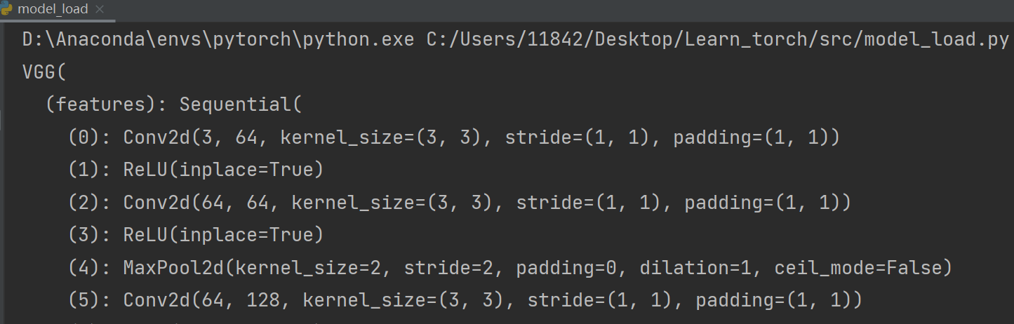
方式1 有陷阱(自己定义网络结构,没有用 vgg16 时)
用方式1保存的话,加载时要让程序能够访问到其定义模型的一种方式
首先在 model_save.py 中写以下代码:
# 陷阱
from torch import nn

class Tudui(nn.Module):
    def __init__(self):
        super(Tudui, self).__init__()
        self.conv = nn.Conv2d(3,64,kernel_size=3)
    def forward(self,x):   # x为输入
        x = self.conv(x)
        return x

tudui = Tudui()  # 有一个卷积层和一些初始化的参数
torch.save(tudui,"tudui_method1.pth")
运行后 src 文件夹底下多出一个文件:

再在 model_load.py 中写以下代码:
# 陷阱
import torch

model = torch.load("tudui_method1.pth")
print(model)
运行后发现报错:

解决:
还是需要将 model_save.py 中的网络结构复制到 model_load.py 中,即下列代码需要复制到 model_load.py 中(为了确保加载的网络模型是想要的网络模型):
class Tudui(nn.Module):
    def __init__(self):
        super(Tudui, self).__init__()
        self.conv = nn.Conv2d(3,64,kernel_size=3)
    def forward(self,x):   # x为输入
        x = self.conv(x)
        return x
但是不需要创建了,即在 model_load.py 中不需要写:
tudui = Tudui()此时 model_load.py 完整代码为:
# 陷阱
class Tudui(nn.Module):
def __init__(self):
super(Tudui, self).__init__()
self.conv = nn.Conv2d(3,64,kernel_size=3)
def forward(self,x): # x为输入
x = self.conv(x)
return x
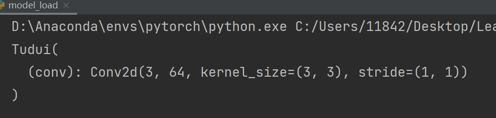
model = torch.load("tudui_method1.pth")
print(model)运行结果如下:
解决另法:
实际写项目过程中,直接定义在一个单独的文件中(如model_save.py),再在 model_load.py 中:
from model_save import *这篇课程的学习和总结到这里就结束啦,如果有什么问题可以在评论区留言呀~
如果帮助到大家,可以一键三连+关注支持下~
学习系列笔记(已完结):
【我是土堆 - Pytorch教程】 知识点 学习总结笔记(一)_耿鬼喝椰汁的博客-CSDN博客
【我是土堆 - Pytorch教程】 知识点 学习总结笔记(二)_耿鬼喝椰汁的博客-CSDN博客
【我是土堆 - Pytorch教程】 知识点 学习总结笔记(三)_耿鬼喝椰汁的博客-CSDN博客