欢迎大家访问个人博客：https://jmxgodlz.xyz

前言

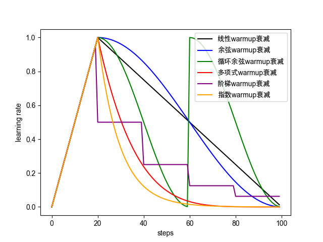
本文将介绍神经网络调参技巧：warmup，decay。反向传播主要完成参数更新： $\theta_t=\theta_{t-1}-\alpha * g_t$ ，其中 $\alpha$ 为学习率， $g_t$ 为梯度更新量，而warmup、decay就是调整 $\alpha$ 的方式，优化器决定梯度更新的方式即 $g_t$ 的计算方式。衰减方式如下图所示：

warmup and decay

定义

Warmup and Decay是模型训练过程中，一种学习率（learning rate）的调整策略。

Warmup是在ResNet论文中提到的一种学习率预热的方法，它在训练开始的时候先选择使用一个较小的学习率，训练了一些epoches或者steps(比如4个epoches,10000steps),再修改为预先设置的学习来进行训练。

同理，Decay是学习率衰减方法，它指定在训练到一定epoches或者steps后，按照线性或者余弦函数等方式，将学习率降低至指定值。一般，使用Warmup and Decay，学习率会遵循从小到大，再减小的规律。

为什么要warmup

这里引用知乎：https://www.zhihu.com/question/338066667/answer/771252708的讨论：
SGD训练中常见的方式是初始较大的学习率，然后衰减为小的学习率，而warmup是先以较小的学习率上升到初始学习率，然后再衰减到小的学习率上，那么为什么warmup有效。

直观上解释

深层网络随机初始化差异较大，如果一开始以较大的学习率，初始学习带来的偏差在后续学习过程中难以纠正。

训练刚开始时梯度更新较大，若学习率设置较大则更新的幅度较大，该类型与传统学习率先大后小方式不同的原因在于起初浅层网络幅度大的更新并不会导致方向错误。

理论上解释

warmup带来的优点包含：

缓解模型在初期对mini-batch过拟合的现象
保持模型深层的稳定性

给出三个论文中的结论：

当batch大小增加时，学习率也可以成倍增加
限制大batch训练的是高学习率带来的训练不稳定性
warmup主要限制深层的权重变化，并且冻结深层权重的变化可以取得相似的效果

batch与学习率大小的关系

假设现在模型已经train到第t步，权重为 $w_t$ ，我们有k个mini-batch，每个mini-batch大小为n，记为 $\mathcal{B}_{1:k}$ 。下面我们来看，以学习率 $\eta$ 训k次 $\mathcal{B}_{1:k}$ 和以学习率 $\hat{\eta}$ 一次训练 $\mathcal{B}$ 时学习率的关系。

假设我们用的是SGD，那么训k次后我们可以得到：
$w_{t+k}=w_{t}-\eta \frac{1}{n} \sum_{j<k} \sum_{x \in \mathcal{B}_{j}} \nabla l\left(x, w_{t+j}\right)$
如果我们一次训练就可以得到：
$\hat{w}_{t+1}=w_{t}-\hat{\eta} \frac{1}{k n} \sum_{j<k} \sum_{x \in \mathcal{B}_{j}} \nabla l\left(x, w_{t}\right)$

其中 $w_{t+k}$ 与 $\hat{w}_{t+1}$ 代表按上述方式训练k次与1次，完成参数更新后的参数。显然，这两个是不一样的。但如果我们假设 $\nabla l\left(x, w_{t}\right) \approx \nabla l\left(x, w_{t+j}\right)$ ，那么令 $\hat{\eta}=k\eta$ 就可以保证 $\hat{w}_{t+1} \approx w_{t+k}$ 。那么，在什么时候 $\nabla l\left(x, w_{t}\right) \approx \nabla l\left(x, w_{t+j}\right)$ 可能不成立呢？[1]告诉我们有两种情况：

在训练的开始阶段，模型权重迅速改变
Mini-batch 大小较小，样本方差较大

第一种情况，模型初始参数分布取决于初始化方式，初始数据对于模型都是初次修正，所以梯度更新较大，若一开始以较大的学习率学习，易对数据造成过拟合，需要经过之后更多轮的训练进行修正。

第二种情况，在训练的过程中，如果有mini-batch内的数据分布方差特别大，这会导致模型学习剧烈波动，使其学得的权重很不稳定，这在训练初期最为明显，最后期较为缓解。

针对上述两种情况，并不能简单的成倍增长学习率 $\hat{\eta}=k\eta$ ,因为此时不符合 $\nabla l\left(x, w_{t}\right) \approx \nabla l\left(x, w_{t+j}\right)$ 假设。此时要么更改学习率增长方式[warmup]，要么解决这两种情况[数据预处理以减小样本方差]。

warmup与模型学习的稳定性

该部分通过一些论文实验结果，推断有了warmup之后模型能够学习的更稳定。

上图表示有了warmup之后，模型能够学习的更加稳定。

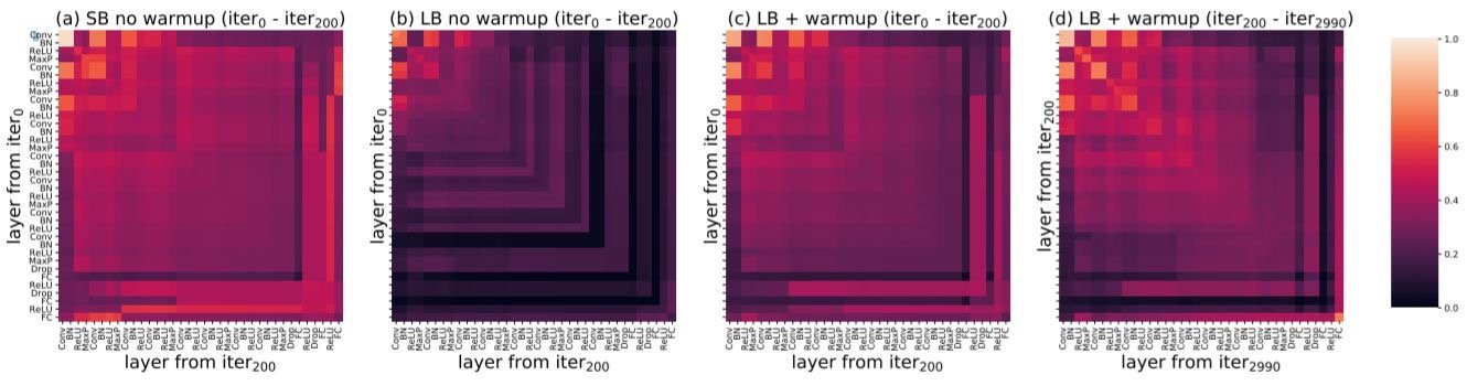
上图b，c表示有了warmup之后，模型最后几层的相似性增加，避免模型不稳定的改变。

学习率衰减策略

可视化代码

下列各种学习率衰减策略均采用warmup，为了图片反应的更加直观：起始学习率设置为1，warmup 步数为20，总步数为100。通常warmup步数可以设置为总步数的10%，参照BERT的经验策略。

#!/usr/bin/env python
# -*- coding: utf-8 -*-
# author： JMXGODLZZ
# datetime： 2022/1/23 下午7:10 
# ide： PyCharm
import keras
import tensorflow as tf
import matplotlib.pyplot as plt

from learningrateSchedules import get_linear_schedule_with_warmup, get_cosine_schedule_with_warmup
from learningrateSchedules import get_cosine_with_hard_restarts_schedule_with_warmup
from learningrateSchedules import get_polynomial_decay_schedule_with_warmup
from learningrateSchedules import get_step_schedule_with_warmup
from learningrateSchedules import get_exp_schedule_with_warmup
init_lr = 1
warmupsteps = 20
totalsteps = 100

lrs = get_linear_schedule_with_warmup(1, warmupsteps, totalsteps)
cos_warm_lrs = get_cosine_schedule_with_warmup(1, warmupsteps, totalsteps)
cos_hard_warm_lrs = get_cosine_with_hard_restarts_schedule_with_warmup(1, warmupsteps, totalsteps, 2)
poly_warm_lrs = get_polynomial_decay_schedule_with_warmup(1, warmupsteps, totalsteps, 0, 5)
step_warm_lrs = get_step_schedule_with_warmup(1, warmupsteps, totalsteps)
exp_warm_lrs = get_exp_schedule_with_warmup(1, warmupsteps, totalsteps, 0.9)
x = list(range(totalsteps))
plt.figure()
plt.plot(x, lrs, label='linear_warmup', color='k')
plt.plot(x, cos_warm_lrs, label='cosine_warmup', color='b')
plt.plot(x, cos_hard_warm_lrs, label='cosine_cy2_warmup', color='g')
plt.plot(x, poly_warm_lrs, label='polynomial_warmup_pw5', color='r')
plt.plot(x, step_warm_lrs, label='step_warmup', color='purple')
plt.plot(x, exp_warm_lrs, label='exp_warmup', color='orange')
plt.xlabel('steps')
plt.ylabel('learning rate')
plt.legend()
plt.show()

指数衰减学习率

def get_exp_schedule_with_warmup(learning_rate, num_warmup_steps, num_training_steps, gamma, last_epoch=-1):
    """
    Create a schedule with a learning rate that decreases linearly from the initial lr set in the optimizer to 0, after
    a warmup period during which it increases linearly from 0 to the initial lr set in the optimizer.

    Args:
        optimizer (:class:`~torch.optim.Optimizer`):
            The optimizer for which to schedule the learning rate.
        num_warmup_steps (:obj:`int`):
            The number of steps for the warmup phase.
        num_training_steps (:obj:`int`):
            The total number of training steps.
        last_epoch (:obj:`int`, `optional`, defaults to -1):
            The index of the last epoch when resuming training.

    Return:
        :obj:`torch.optim.lr_scheduler.LambdaLR` with the appropriate schedule.
    """

    def lr_lambda(current_step: int):
        if current_step < num_warmup_steps:
            return float(current_step) / float(max(1, num_warmup_steps))
        stepmi = (current_step - num_warmup_steps)
        return pow(gamma, stepmi)
    lrs = []
    for current_step in range(num_training_steps):
        cur_lr = lr_lambda(current_step) * learning_rate
        lrs.append(cur_lr)
    return lrs

余弦衰减学习率

def get_cosine_schedule_with_warmup(
    learning_rate, num_warmup_steps: int, num_training_steps: int, num_cycles: float = 0.5, last_epoch: int = -1
):
    """
    Create a schedule with a learning rate that decreases following the values of the cosine function between the
    initial lr set in the optimizer to 0, after a warmup period during which it increases linearly between 0 and the
    initial lr set in the optimizer.

    Args:
        optimizer (:class:`~torch.optim.Optimizer`):
            The optimizer for which to schedule the learning rate.
        num_warmup_steps (:obj:`int`):
            The number of steps for the warmup phase.
        num_training_steps (:obj:`int`):
            The total number of training steps.
        num_cycles (:obj:`float`, `optional`, defaults to 0.5):
            The number of waves in the cosine schedule (the defaults is to just decrease from the max value to 0
            following a half-cosine).
        last_epoch (:obj:`int`, `optional`, defaults to -1):
            The index of the last epoch when resuming training.

    Return:
        :obj:`torch.optim.lr_scheduler.LambdaLR` with the appropriate schedule.
    """

    def lr_lambda(current_step):
        if current_step < num_warmup_steps:
            return float(current_step) / float(max(1, num_warmup_steps))
        progress = float(current_step - num_warmup_steps) / float(max(1, num_training_steps - num_warmup_steps))
        return max(0.0, 0.5 * (1.0 + math.cos(math.pi * float(num_cycles) * 2.0 * progress)))

    lrs = []
    for current_step in range(num_training_steps):
        cur_lr = lr_lambda(current_step) * learning_rate
        lrs.append(cur_lr)
    return lrs

线性衰减学习率

def get_linear_schedule_with_warmup(learning_rate, num_warmup_steps, num_training_steps, last_epoch=-1):
    """
    Create a schedule with a learning rate that decreases linearly from the initial lr set in the optimizer to 0, after
    a warmup period during which it increases linearly from 0 to the initial lr set in the optimizer.

    Args:
        optimizer (:class:`~torch.optim.Optimizer`):
            The optimizer for which to schedule the learning rate.
        num_warmup_steps (:obj:`int`):
            The number of steps for the warmup phase.
        num_training_steps (:obj:`int`):
            The total number of training steps.
        last_epoch (:obj:`int`, `optional`, defaults to -1):
            The index of the last epoch when resuming training.

    Return:
        :obj:`torch.optim.lr_scheduler.LambdaLR` with the appropriate schedule.
    """

    def lr_lambda(current_step: int):
        if current_step < num_warmup_steps:
            return float(current_step) / float(max(1, num_warmup_steps))
        return max(
            0.0, float(num_training_steps - current_step) / float(max(1, num_training_steps - num_warmup_steps))
        )
    lrs = []
    for current_step in range(num_training_steps):
        cur_lr = lr_lambda(current_step) * learning_rate
        lrs.append(cur_lr)
    return lrs

阶梯衰减学习率

def get_step_schedule_with_warmup(learning_rate, num_warmup_steps, num_training_steps, last_epoch=-1):
    """
    Create a schedule with a learning rate that decreases linearly from the initial lr set in the optimizer to 0, after
    a warmup period during which it increases linearly from 0 to the initial lr set in the optimizer.

    Args:
        optimizer (:class:`~torch.optim.Optimizer`):
            The optimizer for which to schedule the learning rate.
        num_warmup_steps (:obj:`int`):
            The number of steps for the warmup phase.
        num_training_steps (:obj:`int`):
            The total number of training steps.
        last_epoch (:obj:`int`, `optional`, defaults to -1):
            The index of the last epoch when resuming training.

    Return:
        :obj:`torch.optim.lr_scheduler.LambdaLR` with the appropriate schedule.
    """

    def lr_lambda(current_step: int):
        if current_step < num_warmup_steps:
            return float(current_step) / float(max(1, num_warmup_steps))
        stepmi = (current_step - num_warmup_steps) // 20 + 1
        return pow(0.5, stepmi)
    lrs = []
    for current_step in range(num_training_steps):
        cur_lr = lr_lambda(current_step) * learning_rate
        lrs.append(cur_lr)
    return lrs

多项式衰减学习率

def get_polynomial_decay_schedule_with_warmup(
    learning_rate, num_warmup_steps, num_training_steps, lr_end=1e-7, power=1.0, last_epoch=-1
):
    """
    Create a schedule with a learning rate that decreases as a polynomial decay from the initial lr set in the
    optimizer to end lr defined by `lr_end`, after a warmup period during which it increases linearly from 0 to the
    initial lr set in the optimizer.

    Args:
        optimizer (:class:`~torch.optim.Optimizer`):
            The optimizer for which to schedule the learning rate.
        num_warmup_steps (:obj:`int`):
            The number of steps for the warmup phase.
        num_training_steps (:obj:`int`):
            The total number of training steps.
        lr_end (:obj:`float`, `optional`, defaults to 1e-7):
            The end LR.
        power (:obj:`float`, `optional`, defaults to 1.0):
            Power factor.
        last_epoch (:obj:`int`, `optional`, defaults to -1):
            The index of the last epoch when resuming training.

    Note: `power` defaults to 1.0 as in the fairseq implementation, which in turn is based on the original BERT
    implementation at
    https://github.com/google-research/bert/blob/f39e881b169b9d53bea03d2d341b31707a6c052b/optimization.py#L37

    Return:
        :obj:`torch.optim.lr_scheduler.LambdaLR` with the appropriate schedule.

    """

    lr_init = learning_rate
    if not (lr_init > lr_end):
        raise ValueError(f"lr_end ({lr_end}) must be be smaller than initial lr ({lr_init})")

    def lr_lambda(current_step: int):
        if current_step < num_warmup_steps:
            return float(current_step) / float(max(1, num_warmup_steps))
        elif current_step > num_training_steps:
            return lr_end / lr_init  # as LambdaLR multiplies by lr_init
        else:
            lr_range = lr_init - lr_end
            decay_steps = num_training_steps - num_warmup_steps
            pct_remaining = 1 - (current_step - num_warmup_steps) / decay_steps
            decay = lr_range * pct_remaining ** power + lr_end
            return decay / lr_init  # as LambdaLR multiplies by lr_init

    lrs = []
    for current_step in range(num_training_steps):
        cur_lr = lr_lambda(current_step) * learning_rate
        lrs.append(cur_lr)
    return lrs

余弦循环衰减学习率

def get_cosine_with_hard_restarts_schedule_with_warmup(
    learning_rate, num_warmup_steps: int, num_training_steps: int, num_cycles: int = 1, last_epoch: int = -1
):
    """
    Create a schedule with a learning rate that decreases following the values of the cosine function between the
    initial lr set in the optimizer to 0, with several hard restarts, after a warmup period during which it increases
    linearly between 0 and the initial lr set in the optimizer.

    Args:
        optimizer (:class:`~torch.optim.Optimizer`):
            The optimizer for which to schedule the learning rate.
        num_warmup_steps (:obj:`int`):
            The number of steps for the warmup phase.
        num_training_steps (:obj:`int`):
            The total number of training steps.
        num_cycles (:obj:`int`, `optional`, defaults to 1):
            The number of hard restarts to use.
        last_epoch (:obj:`int`, `optional`, defaults to -1):
            The index of the last epoch when resuming training.

    Return:
        :obj:`torch.optim.lr_scheduler.LambdaLR` with the appropriate schedule.
    """

    def lr_lambda(current_step):
        if current_step < num_warmup_steps:
            return float(current_step) / float(max(1, num_warmup_steps))
        progress = float(current_step - num_warmup_steps) / float(max(1, num_training_steps - num_warmup_steps))
        if progress >= 1.0:
            return 0.0
        return max(0.0, 0.5 * (1.0 + math.cos(math.pi * ((float(num_cycles) * progress) % 1.0))))

    lrs = []
    for current_step in range(num_training_steps):
        cur_lr = lr_lambda(current_step) * learning_rate
        lrs.append(cur_lr)
    return lrs

学习率衰减实现

Pytorch学习率策略

if args.scheduler == "constant_schedule":
    scheduler = get_constant_schedule(optimizer)

elif args.scheduler == "constant_schedule_with_warmup":
    scheduler = get_constant_schedule_with_warmup(
        optimizer, num_warmup_steps=args.warmup_steps
    )

elif args.scheduler == "linear_schedule_with_warmup":
    scheduler = get_linear_schedule_with_warmup(
        optimizer,
        num_warmup_steps=args.warmup_steps,
        num_training_steps=t_total,
    )

elif args.scheduler == "cosine_schedule_with_warmup":
    scheduler = get_cosine_schedule_with_warmup(
        optimizer,
        num_warmup_steps=args.warmup_steps,
        num_training_steps=t_total,
        num_cycles=args.cosine_schedule_num_cycles,
    )

elif args.scheduler == "cosine_with_hard_restarts_schedule_with_warmup":
    scheduler = get_cosine_with_hard_restarts_schedule_with_warmup(
        optimizer,
        num_warmup_steps=args.warmup_steps,
        num_training_steps=t_total,
        num_cycles=args.cosine_schedule_num_cycles,
    )

elif args.scheduler == "polynomial_decay_schedule_with_warmup":
    scheduler = get_polynomial_decay_schedule_with_warmup(
        optimizer,
        num_warmup_steps=args.warmup_steps,
        num_training_steps=t_total,
        lr_end=args.polynomial_decay_schedule_lr_end,
        power=args.polynomial_decay_schedule_power,
    )

else:
    raise ValueError("{} is not a valid scheduler.".format(args.scheduler))

keras学习率策略

Keras提供了四种衰减策略分别是ExponentialDecay(指数衰减)、 PiecewiseConstantDecay(分段常数衰减) 、 PolynomialDecay(多项式衰减)和InverseTimeDecay(逆时间衰减)。只要在Optimizer中指定衰减策略，一行代码就能实现，在以下方法一中详细介绍。
如果想要自定义学习率的衰减，有第二种方法，更加灵活，需要使用callbacks来实现动态、自定义学习率衰减策略，方法二中将详细介绍。
如果两种方法同时使用，默认优先使用第二种，第一种方法将被忽略。

方法一

指数衰减

lr_scheduler = tf.keras.optimizers.schedules.ExponentialDecay(
    initial_learning_rate=1e-2,
    decay_steps=10000,
    decay_rate=0.96)
optimizer = tf.keras.optimizers.SGD(learning_rate=lr_scheduler)

分段衰减

[0~1000]的steps，学习率为1.0,[10001～9000]的steps，学习率为0.5，其他steps，学习率为0.1

step = tf.Variable(0, trainable=False)
boundaries = [1000, 10000]
values = [1.0, 0.5, 0.1]
learning_rate_fn = tf.keras.optimizers.schedules.PiecewiseConstantDecay(boundaries, values)
lr_scheduler = learning_rate_fn(step)
optimizer = tf.keras.optimizers.SGD(learning_rate=lr_scheduler)

多项式衰减

在10000步中从0.1衰减到0.001，使用开根式( power=0.5)

start_lr = 0.1
end_lr = 0.001
decay_steps = 10000
lr_scheduler = tf.keras.optimizers.schedules.PolynomialDecay(
    start_lr,
    decay_steps,
    end_lr,
    power=0.5)
optimizer = tf.keras.optimizers.SGD(learning_rate=lr_scheduler)

逆时间衰减

initial_lr = 0.1
decay_steps = 1.0
decay_rate = 0.5
lr_scheduler = keras.optimizers.schedules.InverseTimeDecay(
  initial_lr, decay_steps, decay_rate)
optimizer = tf.keras.optimizers.SGD(learning_rate=lr_scheduler)

方法二

自定义指数衰减

# 第一步：自定义指数衰减策略
def step_decay(epoch):
    init_lr = 0.1
    drop=0.5
    epochs_drop=10
    if epoch<100:
        return init_lr
    else:
        return init_lr*pow(drop,floor(1+epoch)/epochs_drop)
        
# ……
# 第二步：用LearningRateScheduler封装学习率衰减策略
lr_callback = LearningRateScheduler(step_decay)
# 第三步：加入callbacks
model = KerasClassifier(build_fn = create_model,epochs=200,batch_size=5,verbose=1,callbacks=[checkpoint,lr_callback])
model.fit(X,Y)

动态修改学习率

ReduceLROnPlateau(monitor=‘val_acc’, mode=‘max’,min_delta=0.1,factor=0.2,patience=5, min_lr=0.001)

训练集连续patience个epochs的val_acc小于min_delta时，学习率将会乘以factor。mode可以选择max或者min，根据monitor的选择而灵活设定。min_lr是学习率的最低值。

# 第一步：ReduceLROnPlateau定义学习动态变化策略
reduce_lr_callback = ReduceLROnPlateau(monitor='val_acc', factor=0.2,patience=5, min_lr=0.001)
# 第二步：加入callbacks
model = KerasClassifier(build_fn = create_model,epochs=200,batch_size=5,verbose=1,callbacks=[checkpoint,reduce_lr_callback])
model.fit(X,Y)

Keras学习率回显代码

def get_lr_metric(optimizer):
    def lr(y_true, y_pred):
        return optimizer.lr
    return lr
 
x = Input((50,))
out = Dense(1, activation='sigmoid')(x)
model = Model(x, out)
 
optimizer = Adam(lr=0.001)
lr_metric = get_lr_metric(optimizer)
model.compile(loss='binary_crossentropy', optimizer=optimizer, metrics=['acc', lr_metric])
 
# reducing the learning rate by half every 2 epochs
cbks = [LerningRateScheduler(lambda epoch: 0.001 * 0.5 ** (epoch // 2)),
        TensorBoard(write_graph=False)]
X = np.random.rand(1000, 50)
Y = np.random.randint(2, size=1000)
model.fit(X, Y, epochs=10, callbacks=cbks)

分层学习率设置

有时候我们需要为模型中不同层设置不同学习率大小，比如微调预训练模型时，预训练层数设置较小的学习率进行学习，而其他层以正常大小进行学习。这里给出苏神给出的keras实现，其通过参数变换实现调整学习率的目的：

梯度下降公式如下：
$\boldsymbol{\theta}_{n+1}=\boldsymbol{\theta}_{n}-\alpha \frac{\partial L(\boldsymbol{\theta}_{n})}{\partial \boldsymbol{\theta}_n}$
考虑变换 $\boldsymbol{\theta}=\lambda \boldsymbol{\phi}$ ,其中λ是一个固定的标量，ϕ也是参数。现在来优化ϕ，相应的更新公式为：
$\begin{aligned}\boldsymbol{\phi}_{n+1}=&\boldsymbol{\phi}_{n}-\alpha \frac{\partial L(\lambda\boldsymbol{\phi}_{n})}{\partial \boldsymbol{\phi}_n}\\ =&\boldsymbol{\phi}_{n}-\alpha \frac{\partial L(\boldsymbol{\theta}_{n})}{\partial \boldsymbol{\theta}_n}\frac{\partial \boldsymbol{\theta}_{n}}{\partial \boldsymbol{\phi}_n}\\ =&\boldsymbol{\phi}_{n}-\lambda\alpha \frac{\partial L(\boldsymbol{\theta}_{n})}{\partial \boldsymbol{\theta}_n}\end{aligned}$
然后通过链式求导法则，再上述等式两边同时乘以λ：
$\lambda\boldsymbol{\phi}_{n+1}=\lambda\boldsymbol{\phi}_{n}-\lambda^2\alpha \frac{\partial L(\boldsymbol{\theta}_{n})}{\partial \boldsymbol{\theta}_n}\quad\Rightarrow\quad\boldsymbol{\theta}_{n+1}=\boldsymbol{\theta}_{n}-\lambda^2\alpha \frac{\partial L(\boldsymbol{\theta}_{n})}{\partial \boldsymbol{\theta}_n}$

在SGD优化器中，如果做参数变换θ=λϕ，那么等价的结果是学习率从α变成了 $\lambda^2\alpha$ 。

不过，在自适应学习率优化器（比如RMSprop、Adam等），情况有点不一样，因为自适应学习率使用梯度（作为分母）来调整了学习率，抵消了一个λ

在RMSprop、Adam等自适应学习率优化器中，如果做参数变换θ=λϕ，那么等价的结果是学习率从α变成了λα。

import keras.backend as K

class SetLearningRate:
    """层的一个包装，用来设置当前层的学习率
    """

    def __init__(self, layer, lamb, is_ada=False):
        self.layer = layer
        self.lamb = lamb # 学习率比例
        self.is_ada = is_ada # 是否自适应学习率优化器

    def __call__(self, inputs):
        with K.name_scope(self.layer.name):
            if not self.layer.built:
                input_shape = K.int_shape(inputs)
                self.layer.build(input_shape)
                self.layer.built = True
                if self.layer._initial_weights is not None:
                    self.layer.set_weights(self.layer._initial_weights)
        for key in ['kernel', 'bias', 'embeddings', 'depthwise_kernel', 'pointwise_kernel', 'recurrent_kernel', 'gamma', 'beta']:
            if hasattr(self.layer, key):
                weight = getattr(self.layer, key)
                if self.is_ada:
                    lamb = self.lamb # 自适应学习率优化器直接保持lamb比例
                else:
                    lamb = self.lamb**0.5 # SGD（包括动量加速），lamb要开平方
                K.set_value(weight, K.eval(weight) / lamb) # 更改初始化
                setattr(self.layer, key, weight * lamb) # 按比例替换
        return self.layer(inputs)
 
x_in = Input(shape=(None,))
x = x_in

# 默认情况下是x = Embedding(100, 1000, weights=[word_vecs])(x)
# 下面这一句表示：后面将会用自适应学习率优化器，并且Embedding层以总体的十分之一的学习率更新。
# word_vecs是预训练好的词向量
x = SetLearningRate(Embedding(100, 1000, weights=[word_vecs]), 0.1, True)(x)

# 后面部分自己想象了～
x = LSTM(100)(x)

model = Model(x_in, x)
model.compile(loss='mse', optimizer='adam') # 用自适应学习率优化器优化

参考文献

https://jishuin.proginn.com/p/763bfbd51f6b

https://www.zhihu.com/question/338066667/answer/771252708

https://kexue.fm/archives/6418

神经网络调参-warmup and decay

前言