基于Orfeo ToolBox+TensorFlow 遥感影像分类教程

一、前言

在本博客中，我们将了解如何仅使用面向用户的开源软件在真实世界的遥感图像上训练和应用深度神经网络。 无需编码技能！

我们想要对 Sentinel-2 图像进行分类，这意味着我们打算估计每个像素的类别。 由于我们的地形真实数据被稀疏地注释，我们的方法包括训练一个网络来估计特定图像块的一个单一类值。 如果我们有一个密集注释的数据集，我们可以使用语义分割方法。我们将使用 Orfeo ToolBox 的 OTBTF 远程模块。 OTBTF 依靠 TensorFlow 来执行数值计算。

二、数据处理

（1）数据介绍

我们的“东京数据集”是免费提供的。 它的组成如下：

• 一张 Sentinel-2 图像，可以从欧洲航天局中心或您首选的 Sentinel 访问门户下载。 只需下载名为 S2A_MSIL2A_20190508T012701_N0212_R074_T54SUE_20190518T165701 的 2019/05/08（任务：Sentinel-2，平台：S2A_*）在东京市上空获取的 Sentinel-2 图像。

• 两张真实地形标签图像（一张用于训练，一张用于验证）。 每个像素要么是“无数据”值 (255)，要么是类值（从 0 开始）。

在以下步骤中，我们建议您使用 QGIS 检查生成的地理空间数据。 请注意，应用程序参数以命令行的形式提供，但可以使用 OTB 的图形用户界面执行！

我们可以分解我们将执行的步骤如下：

• 采样：我们提取与地形真实相关的图像块，

• 训练：我们从补丁中训练模型，

• 推理：将模型应用于完整图像，生成漂亮的土地覆盖图！

（2）数据标准化

我们将使用 BandMathX 堆叠和规范化 Sentinel-2 图像。 我们将图像归一化，例如像素值在 [0,1] 区间内。

ng images (Tutorial)
Update (28/01/2020): open dataset, available for download!

In this tutorial, we will see how to train and apply a deep neural network on real world remote sensing images, using only user-oriented open-source software. No coding skills required!

Data
Our “Tokyo dataset” is freely available. It is composed as follow:

One Sentinel-2 image, that can be downloaded from the European Space Agency hub or from your preferred Sentinel access portal. Just download the Sentinel-2 image acquired over the city of Tokyo the 2019/05/08 (Mission: Sentinel-2, Platform: S2A_*) named S2A_MSIL2A_20190508T012701_N0212_R074_T54SUE_20190518T165701.
Two label images of terrain truth (one for training and one for validation). Each pixel is either a “no-data” value (255) or a class value (starting from 0). The files can be downloaded here (also provided: the style .qml file for QGIS). This dataset has been elaborated for educational purpose at our research facility, using Open Street Map data.
Goal
We want to classify the Sentinel-2 image, meaning that we intend to estimate the class for each pixel. Since our terrain truth data is sparsely annotated, our approach consist in training a network that estimates one single class value for a particular patch of image. If we had a densely annotated dataset, we could have used the semantic segmentation approach, but this will be another story (soon on this blog!).

We will use the OTBTF remote module of the Orfeo ToolBox. OTBTF relies on TensorFlow to perform numeric computations. You can read more about OTBTF on the blog post here.


OTBTF = Orfeo ToolBox (OTB) + TensorFlow (TF)
It is completely user-oriented, and you can use the provided applications in graphical user interface as any Orfeo ToolBox applications. Concepts introduced in OTBTF are presented in [1]. The easiest way to install and begin with OTBTF is to use the provided docker images.

Deep learning backgrounds
To goal of this post is not to do a lecture about how deep learning works, but quickly summarizing the principle!

Deep learning refers to artificial neural networks with deep neuronal layers (i.e. a lot of layers !). Artificial neurons and edges typically have parameters that adjust as learning proceeds.

Weights modify the strength of the signal at a connection. Artificial neurons may output in non linear functions to break the linearity, for instance to make the signal sent only if the aggregate signal crosses a given threshold. Typically, artificial neurons are aggregated into layers. Different layers may perform different kinds of transformations on their inputs. Signals travel from the first layer (the input layer), to the last layer (the output layer), possibly after traversing the layers multiple times. Among common networks, Convolutional Neural Networks (CNN) achieve state of the art results on images. CNN are designed to extract features, enabling image recognition, object detection, semantic segmentation. A good review of deep learning techniques applied to remote sensing can be found here [2]. In this tutorial, we focus only on CNN for a sake of simplicity.

Let’s start
During the following steps, we advise you to use QGIS to check generated geospatial data. Note that applications parameters are provided in the form of command line, but can be performed using the graphical user interface of OTB!

We can decompose the steps that we will perform as follow:

Sampling: we extract patches of images associated to the terrain truth,
Training: we train the model from patches,
Inference: Apply the model to the full image, to generate a nice landcover map!
Normalize the remote sensing images
We will stack and normalize the Sentinel-2 images using BandMathX. We normalize the images such as the pixels values are within the [0,1]  interval. 

# Go in S2 folder
cd S2A_MSIL2A_20190508T012701_N0212_R074_T54SUE_20190508T041235.SAFE
cd GRANULE/L2A_T54SUE_A020234_20190508T012659/IMG_DATA/R10m/

# Apply BandMathX
otbcli_BandMathX \
-il T54SUE_20190508T012701_B04_10m.jp2 \
    T54SUE_20190508T012701_B03_10m.jp2 \
    T54SUE_20190508T012701_B02_10m.jp2 \
    T54SUE_20190508T012701_B08_10m.jp2 \
-exp "{im1b1/im1b1Maxi;im2b1/im2b1Maxi;im3b1/im3b1Maxi;im4b1/im4b1Maxi}" \
-out Sentinel-2_B4328_10m.tif

（3）对遥感图像进行采样

将深度学习技术应用于现实世界数据集的第一步是采样。 OTB 的现有框架为像素级或面向对象的分类/回归任务提供了很好的工具。 在深度学习方面，像 CNN 这样的网络是在图像块而不是单个像素的批次上训练的。 因此，我们将介绍的 OTBTF 的第一个应用程序以补丁采样为目标，称为 PatchesExtraction。

PatchesExtraction 应用程序无缝集成到 OTB 的现有采样框架中。 通常，我们有两种选择，具体取决于我们的地形真实情况是矢量数据还是标签图像。

• 矢量数据：可以使用 PolygoncClassStatistics（计算输入地形真相的一些统计数据）和 SampleSelection 应用程序来选择补丁位置，然后将它们提供给 PatchesExtraction 应用程序。

• 标签图像：我们可以直接使用 OTBTF 中的 LabelImageSampleSelection 应用程序来选择补丁位置。

在我们的例子中，我们有标签图像形式的地形真相。 因此，我们将使用选项 2。让我们使用以下命令行为每个类选择 500 个样本：

# Samples selection for group A
otbcli_LabelImageSampleSelection \
-inref ~/tokyo/terrain_truth/terrain_truth_epsg32654_A.tif \
-nodata 255 \
-outvec terrain_truth_epsg32654_A_pos.shp \
-strategy "constant" \
-strategy.constant.nb 500

• inref 是标签图像，

• nodata 是“无数据”的值（即此位置没有可用的注释），

• strategy 是选择样本位置的策略，

• outvec 是生成的包含样本位置的输出矢量数据的文件名。

对第二个标签图像 (terrain_truth_epsg32654_B.tif) 重复前面描述的步骤。 在 QGIS 中打开数据以检查样本位置是否正确生成。

（4）影像小块提取

现在我们应该有两个向量层：

• terrain_truth_epsg32654_A_pos.shp

• terrain_truth_epsg32654_B_pos.shp

是时候使用 PatchesExtraction 应用程序了。 以下操作包括在 terrain_truth_epsg32654_A_pos.shp 的每个位置提取输入图像中的补丁。 为了稍后训练一个小型 CNN，我们将创建一组尺寸为 16×16 的补丁，这些补丁与矢量数据的类字段中给出的相应标签相关联。 我们开工吧 ：

# Patches extraction
otbcli_PatchesExtraction \
-source1.il Sentinel-2_B4328_10m.tif \
-source1.patchsizex 16 \
-source1.patchsizey 16 \
-source1.out Sentinel-2_B4328_10m_patches_A.tif \
-vec terrain_truth_epsg32654_A_pos.shp \
-field "class" \
-outlabels Sentinel-2_B4328_10m_labels_A.tif uint8

• source1 是第一个图像源（它是一个参数组），

• source1.il是第一个源的输入图像列表，

• source1.patchsizex 是第一个源的补丁宽度，

• source1.patchsizey 是第一个源的补丁高度，

• source1.out 是第一个源的输出补丁图像，

• vec 是点（样本位置）的输入向量数据，

• 字段是我们将用作标签值（即类）的属性，

• outlabels 是标签的输出图像（我们可以强制像素编码为 8 位，因为我们只需要加一个小的正整数）。

在这一步之后，您应该已经生成了以下输出图像，我们将其命名为“训练数据集”：

• Sentinel-2_B4328_10m_patches_A.tif

• Sentinel-2_B4328_10m_labels_A.tif

对矢量图层 terrain_truth_epsg32654_B_pos.shp 重复前面描述的步骤，并生成用于验证的补丁和标签。 在此步骤之后，您应该拥有以下我们将命名为“验证数据集”的数据：

• Sentinel-2_B4328_10m_patches_B.tif

• Sentinel-2_B4328_10m_labels_B.tif

三、开始训练

如何训练深度网络？ 从简单的事情开始，我们将训练一个现有的小型模型。 我们专注于一个 CNN，它输入我们的 16 × 16 × 4 块，并在 0 到 5 的 6 个标签中产生输出类别的预测。

（1）模型

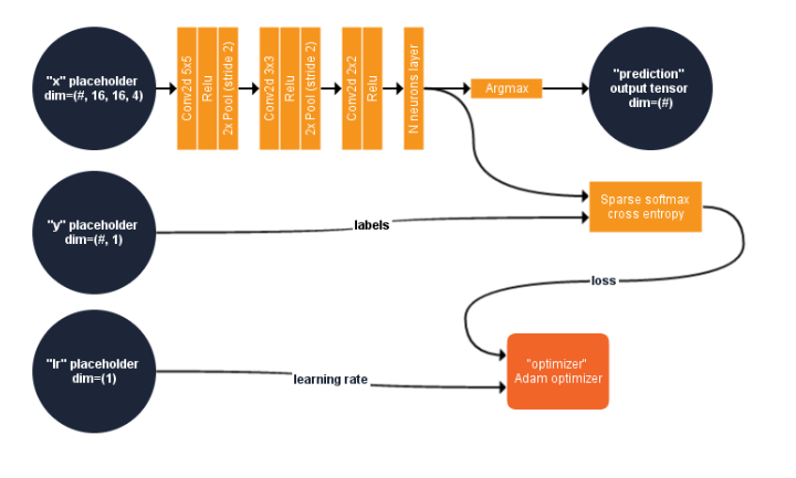
我们建议引入一个小而简单的 CNN 以更好地理解该方法。 本节介绍此模型的内容。 下图总结了我们CNN的计算图。

• 输入：图像块提供了 TensorFlow 模型中名为“x”的占位符。 “x”的第一个维度可能有任意数量的分量。 此维度通常用于批量大小，并不固定以启用不同的批量大小。 例如，假设我们想用一批 10 个样本训练我们的模型，我们将在大小为 # × 16 × 16 × 4 的占位符“x”中为模型提供一个大小为 10 × 16 × 16 × 4 的多维数组。

• 深度网络：“x”然后由一系列二维卷积/激活函数（线性整流）/池化层处理。 在最后一个激活函数之后，特征由 6 个神经元（每个预测类别一个）的全连接层处理。

• 预测类：预测类是输出最大值的神经元（来自最后一层神经元）的索引。 这是在使用 Argmax 运算符处理最后一个完全连接层的输出时执行的，在图中称为“预测”。

• 成本函数：训练的目标是最小化数据分布（真实标签）和模型分布（估计标签）之间的交叉熵。 我们使用 6 个神经元的 softmax 的交叉熵作为成本函数。 简而言之，这将衡量类别互斥（每个条目恰好属于一个类别）的离散分类任务中的概率误差。 为此，该模型实现了一个 TensorFlow 函数，称为 Softmax 交叉熵与对数。 该函数首先计算 6 个神经元输出的 Softmax 函数。 softmax 函数将输出归一化，例如它们的总和等于 1，可用于表示分类分布，即 n 个不同可能结果的概率分布。 然后计算真实标签和来自 softmax 的类概率值之间的香农交叉熵，并将其视为深度网络的损失函数。

• 优化器：关于训练，一个叫做“优化器”的节点执行损失函数的梯度下降：这个节点将仅用于训练（或微调）模型，为模型提供推理是没有用的！ 在此算子中实现的方法称为 Adam（。 名为“lr”的占位符控制优化器的学习率：它包含一个标量值（浮点数）并且可以有一个默认值。

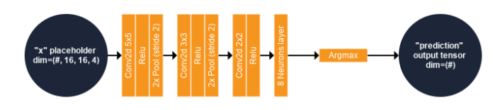
上图为我们的第一个 CNN 架构！

该网络由两个占位符（“x”和“lr”）组成，分别用于输入补丁（4 维数组）和学习率（单标量），一个输出张量（“预测”，一维数组）和一个目标节点（ “优化器”，仅用于训练网络）。 “#”表示第一个维度的分量个数不固定。

要生成此模型，只需将以下内容复制并粘贴到名为 create_model1.py 的 python 脚本中

from tricks import *
import sys
import os

nclasses=6

def myModel(x):
  
  # input patches: 16x16x4
  conv1 = tf.layers.conv2d(inputs=x, filters=16, kernel_size=[5,5], padding="valid", 
                           activation=tf.nn.relu) # out size: 12x12x16
  pool1 = tf.layers.max_pooling2d(inputs=conv1, pool_size=[2, 2], strides=2) # out: 6x6x16
  conv2 = tf.layers.conv2d(inputs=pool1, filters=16, kernel_size=[3,3], padding="valid", 
                           activation=tf.nn.relu) # out size: 4x4x16
  pool2 = tf.layers.max_pooling2d(inputs=conv2, pool_size=[2, 2], strides=2) # out: 2x2x16
  conv3 = tf.layers.conv2d(inputs=pool2, filters=32, kernel_size=[2,2], padding="valid",
                           activation=tf.nn.relu) # out size: 1x1x32
  
  # Features
  features = tf.reshape(conv3, shape=[-1, 32], name="features")
  
  # neurons for classes
  estimated = tf.layers.dense(inputs=features, units=nclasses, activation=None)
  estimated_label = tf.argmax(estimated, 1, name="prediction")

  return estimated, estimated_label
 
""" Main """
if len(sys.argv) != 2:
  print("Usage : <output directory for SavedModel>")
  sys.exit(1)

# Create the TensorFlow graph
with tf.Graph().as_default():
  
  # Placeholders
  x = tf.placeholder(tf.float32, [None, None, None, 4], name="x")
  y = tf.placeholder(tf.int32  , [None, None, None, 1], name="y")
  lr = tf.placeholder_with_default(tf.constant(0.0002, dtype=tf.float32, shape=[]),
                                   shape=[], name="lr")
  
  # Output
  y_estimated, y_label = myModel(x)
  
  # Loss function
  cost = tf.losses.sparse_softmax_cross_entropy(labels=tf.reshape(y, [-1, 1]), 
                                                logits=tf.reshape(y_estimated, [-1, nclasses]))
  
  # Optimizer
  optimizer = tf.train.AdamOptimizer(learning_rate=lr, name="optimizer").minimize(cost)
  
  # Initializer, saver, session
  init = tf.global_variables_initializer()
  saver = tf.train.Saver( max_to_keep=20 )
  sess = tf.Session()
  sess.run(init)

  # Create a SavedModel
  CreateSavedModel(sess, ["x:0", "y:0"], ["features:0", "prediction:0"], sys.argv[1])

导入的 tricks.py 是 OTBTF 远程模块的一部分，包含一组有用的函数和帮助程序来创建 SavedModel 。 它位于 OTBTF 源代码中。 因此，环境变量 PYTHONPATH 必须包含此目录的路径才能在我们的脚本中使用 tricks.py。 我们的 python 脚本使用 TensorFlow python API 生成模型，并将其序列化为写入磁盘的 SavedModel (google protobuf)。

您最终可以使用以下方法生成 SavedModel：

python create_model1.py data/results/SavedModel_cnn

（2）从头开始训练

如果您查看 data/results/SavedModel_cnn 目录，您将看到一个 .pb 文件和一个 Variables 文件夹。 protobuf 文件序列化计算图，Variables 文件夹包含模型权重（内核等）的值。 正如您在 python 脚本中注意到的那样，模型权重在导出 SavedModel 之前进行了初始化。 我们将使用 TensorflowModelTrain 应用程序从其初始化状态训练 CNN，为图像分类任务更新其权重。 对于每个数据集（训练数据和验证数据），TensorflowModelTrain 应用程序的验证步骤包括计算通常的验证指标。

让我们快速总结一下应用程序参数：

• training.source1 是补丁源的参数组（用于学习）

• training.source1.il 是补丁的输入图像文件名

• training.source1.patchsizex 是补丁宽度

• training.source1.patchsizey 是补丁高度

• training.source1.placeholder 是补丁的占位符名称

• training.source2 是标签源的参数组（用于学习）

• training.source2.il 是标签的输入图像文件名

• training.source2.patchsizex 是标签宽度

• training.source2.patchsizey 是标签高度

• training.source2.placeholder 是标签的占位符名称

• model.dir 是包含 TensorFlow SavedModel 的目录

• training.targetnodes 是我们要为训练步骤计算的运算符的名称。 在我们的模型中，梯度下降是通过称为“optimizer”的 adam 优化器节点完成的。

• validation.mode 是验证模式。 “类”验证模式可以计算机器人训练数据和验证数据的分类指标。

• validation.source1 是补丁源的参数组（用于验证）。 由于验证源的名称 (validation.source1.name) 与同一训练源 (training.source1.placeholder) 的占位符名称相同，因此该源被视为模型的输入，并被馈送 在验证步骤期间到相应的占位符。

• validation.source2 是标签源（用于验证）。 由于源名称 (validation.source2.name) 不同于用于训练的相同源 (training.source2.placeholder) 的占位符名称，因此该源被视为要与模型输出进行比较的参考 在验证步骤中具有相同的张量名称。

• model.saveto 可以将模型变量（即权重）导出到文件

上面描述对应的命令行如下：

# Train the deep learning model
otbcli_TensorflowModelTrain \
-training.source1.il Sentinel-2_B4328_10m_patches_A.tif \
-training.source1.patchsizex 16 \
-training.source1.patchsizey 16 \
-training.source1.placeholder "x" \
-training.source2.il Sentinel-2_B4328_10m_labels_A.tif \
-training.source2.patchsizex 1 \
-training.source2.patchsizey 1 \
-training.source2.placeholder "y" \
-model.dir "data/results/SavedModel_cnn" \
-training.targetnodes "optimizer" \
-validation.mode "class" \
-validation.source1.il Sentinel-2_B4328_10m_patches_B.tif \
-validation.source1.name "x" \
-validation.source2.il Sentinel-2_B4328_10m_labels_B.tif \
-validation.source2.name "prediction" \
-model.saveto "data/results/SavedModel_cnn/variables/variables"

运行 TensorflowModelTrain 应用程序。 在 epochs 之后，注意 kappa 和整体准确度指数（在验证数据集上应该分别约为 0.7）。 浏览文件系统，查看 data/results 目录：您可以注意到应用程序更新了两个文件：

• variables.index 是保存变量的汇总，

• variables.data-xxxxx-of-xxxxx 是保存的变量（TensorflowModelTrain 在训练过程结束时只保存了一次）。

（3）运行模型

为此，我们将使用 TensorflowModelServe 应用程序。 我们知道我们的 CNN 输入有一个 16×16 像素的感受野，占位符名称是“x”。 模型的输出是估计的类别，即 Argmax 算子的张量结果，称为“预测”。 在这里，我们不会使用优化器节点，因为它是训练过程的一部分。

对于推理，我们只使用占位符（“x”，我们计算一个名为（“预测”，一维数组）的输出张量。

由于我们目前可能没有 GPU 支持，因此处理整个图像可能会很慢。 我们不会在整个图像上生成地图（即使由于流机制而可能），而只是在一小部分上生成地图。 我们使用输出图像的扩展文件名来执行此操作，设置一个子集，从像素 1000、4000 开始，大小为 1000 × 1000。此扩展文件名包括添加 ?&box=1000 :4000 :1000 :1000 到输出图像文件名。 请注意，您还可以使用 OTB 的 ExtractROI 应用程序生成一个小图像子集，然后将其用作 TensorflowModelServe 应用程序的输入。

otbcli_TensorflowModelServe \
-source1.il Sentinel-2_B4328_10m.tif \
-source1.rfieldx 16 \
-source1.rfieldy 16 \
-source1.placeholder "x" \
-model.dir "data/results/SavedModel_cnn" \
-output.names "prediction" \
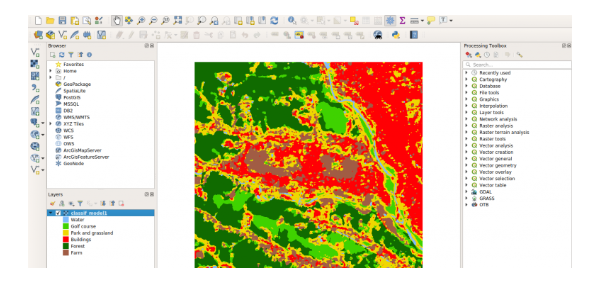
-out "classif_model1.tif?&box=4000:4000:1000:1000"

（4）结果生成

现在将生成的图像导入 QGIS 中。 您可以更改光栅的样式：在图层面板（窗口左侧）中，右键单击图像然后选择属性，然后导入提供的 legend_style.qml 文件。

四、结论

本教程解释了如何使用简单的深度学习架构执行图像分类。

OTBTF 是 Orfeo ToolBox (OTB) 的远程模块，已用于从用户的角度处理图像：本教程不需要任何编码技能。 QGIS 用于可视化目的。