前言
LightGCN原理请参考上一篇博客:推荐系统笔记(五):lightGCN算法原理与背景_甘霖那的博客-CSDN博客
实现
步骤一:建立一个类将数据转化为float tensor类型的数据,便捷进行数据转换:
class Train_data(Dataset):
    def __init__(self, data):
        super(Train_data,self).__init__()
        self.S = torch.tensor(data).float()

    def __len__(self):
        return len(self.S)

    def __getitem__(self, index):
return self.S[index]步骤二:数据集处理,数据集下载链接:MovieLens | GroupLens
import pandas as pd
import numpy as np

df = pd.read_csv('ratings.csv')
users=set(df['userId'].tolist())
movies=set(df['movieId'].tolist())
print("一共有{}条数据 {}个用户 {}部电影".format(len(df),len(users),len(movies)))
print("评分在0~1之间有{}条数据".format(len(df.loc[(df['rating']>=0.0)&(df['rating']<=1.0)])))
print("评分在1~2之间有{}条数据".format(len(df.loc[(df['rating']>1.0)&(df['rating']<=2.0)])))
print("评分在2~3之间有{}条数据".format(len(df.loc[(df['rating']>2.0)&(df['rating']<=3.0)])))
print("评分在3~4之间有{}条数据".format(len(df.loc[(df['rating']>3.0)&(df['rating']<=4.0)])))
print("评分在4~5之间有{}条数据".format(len(df.loc[(df['rating']>4.0)&(df['rating']<=5.0)])))


df.sort_values("movieId", inplace=True)
pointer=0
movies=sorted(movies)
for i in movies:
    df.loc[df['movieId'] == i,'movieId']=pointer
    pointer+=1

with open("train.txt", "w") as f1:
    with open("test.txt", "w") as f2:
        for i in range(0,len(users),1):
            temp_list=df.loc[df['userId']==i+1]
            temp_list=temp_list.sample(frac=1,random_state=2022)
            train_list=pd.concat(np.array_split(temp_list,10)[0:8],axis=0).sort_values(by='rating',ascending=False)
            test_list=pd.concat(np.array_split(temp_list,10)[8:],axis=0).sort_values(by='rating',ascending=False)
            train=train_list['movieId'].tolist()
            test=test_list['movieId'].tolist()
            f1.write(str(i)+' '+(str(train).replace('[','').replace(']','')).replace("'",'').replace(',','') +'\n')
            f2.write(str(i)+' '+(str(test).replace('[','').replace(']','')).replace("'",'').replace(',','') +'\n')
    f2.close()
f1.close()
数据集包含的links包含的是不同的url对电影的标签,这在readme.txt文件里有所介绍。movies.csv文件里包含的是电影标签、标题和电影类型,rating则包含的是用户对电影的评分,数据是整数,tags是用户对电影的评价。我们需要将其转化为类似下面的数据:
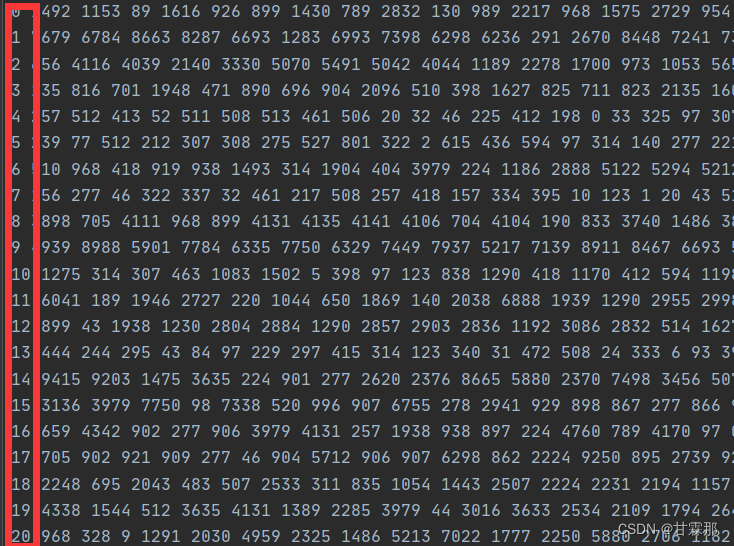
第一列数据是用户ID,后边的是items即电影的ID,因为数据集是稀疏的,这里对其进行了重新排序。即从1~10000按照顺序排列。最后形成一个训练集一个测试集:

步骤三:搭建网络
1. 数据初始化:我们的的参数是输入的embedding数据,因此需要初始化,这里使用了正态分布初始化。
class LightGCN(nn.Module):
    def __init__(self,fname, lamda = 1e-4, lr = 3e-4, latent_dim = 64, device = torch.device('cpu')):
        super(LightGCN, self).__init__()

        self.device = device

        self.mat = self.load_data(fname).to(self.device)

        # print("graph", self.mat.shape)

        self.logger = Logger()

        self.lamda = lamda
        self.user_emb = nn.Embedding(self.n_users, latent_dim).double()
        self.item_emb = nn.Embedding(self.n_items, latent_dim).double()

        nn.init.normal_(self.user_emb.weight, std=0.1)
        nn.init.normal_(self.item_emb.weight, std=0.1)

        self.optimizer = Adam(self.parameters(), lr = lr)
2. 设计BPR loss损失函数进行优化,BPR loss的原理请参考我的另外一篇博客BPR loss
    def bpr_loss(self, S, emb, init_emb):

        S = np.array(S).astype('int')

        all_user_emb, all_item_emb = torch.split(emb,[self.n_users,self.n_items])
        all_user_emb0, all_item_emb0 = torch.split(init_emb,[self.n_users,self.n_items])

        pos_emb = all_item_emb[S[:,1]]
        neg_emb = all_item_emb[S[:,2]]
        user_emb = all_user_emb[S[:,0]]

        #print("pos norm",torch.norm(pos_emb).item())
        #print("neg norm",torch.norm(neg_emb).item())
        #print("user norm",torch.norm(user_emb).item())

        pos_emb0 = all_item_emb0[S[:,1]]
        neg_emb0 = all_item_emb0[S[:,2]]
        user_emb0 = all_user_emb0[S[:,0]]

        loss = (F.softplus(torch.sum(user_emb*neg_emb, dim = 1) - torch.sum(user_emb*pos_emb, dim =1))).mean()

        #print("loss1",loss.item())

        loss += self.lamda*(torch.norm(pos_emb0)**2 + torch.norm(neg_emb0)**2 + torch.norm(user_emb0)**2)/float(len(pos_emb))

        #print("loss total",loss.item())

        return loss
3. 训练数据集的集成,或者说bootstrap,因为数据集应该是一个三元组,所以需要我们选择一个positive example和一个negative example进行数据集成,因此我们需要随机选取并且构建coo_matrix构建邻接矩阵和度矩阵:
    def load_data(self,fname):

        file = open(fname,'r')
        train = {}
        users = set()
        items = set()
        self.n_users = 0
        self.n_items = 0
        count = 0

        self.n_interaction = 0

        while True:
            line = file.readline()[:-1]
            if(line == ''):
                break
            temp = line.split(' ')
            temp = list(map(lambda x: int(x),temp))

            count += (len(temp) -1)

            users.add(temp[0])

            self.n_interaction += len(temp[1:])

            items = items.union(set(temp[1:]))

            if(train.get(temp[0]) is None):
                train[temp[0]] = []
                train[temp[0]].extend(temp[1:])
            else:
                train[temp[0]].extend(temp[1:])
            self.n_users = max(self.n_users,temp[0]+1)
            self.n_items = max(self.n_items,max(temp[1:])+1)
        self.train = train
        self.users = users
        self.items = items
        # print(self.n_users)
        # print(self.n_items)
        row_arr = np.zeros(2*count, dtype = np.int32)
        col_arr = np.zeros(2*count, dtype = np.int32)
        data = np.ones(2*count, dtype = np.int32)

        # self.n_users = len(users)
        # self.n_items = len(items)
        # print("user:{} item:{}".format(len(users),len(items)))
        count = 0
        for key in train.keys():
            for value in train[key]:
                row_arr[count] = int(key)
                col_arr[count] = len(users)+int(value)
                count+=1

        for key in train.keys():
            for value in train[key]:
                row_arr[count] = len(users) + int(value)
                col_arr[count] = int(key)
                count+=1

        mat = coo_matrix((data,(row_arr,col_arr)))
        np.seterr(divide='ignore', invalid='ignore')

        d_mat = mat.sum(axis = 1)
        d_mat = np.sqrt(d_mat)
        d_mat = np.array(d_mat)
        d_mat = 1/(d_mat.reshape(-1))
        d_mat = diags(d_mat)
        d_mat = d_mat.tocoo()
        final = (d_mat@mat@d_mat).tocoo()
        # print(final.shape)

        rows = torch.tensor(final.row)
        cols = torch.tensor(final.col)
        index = torch.cat([rows.reshape(1,-1), cols.reshape(1,-1)], axis = 0)
        return torch.sparse_coo_tensor(index,torch.tensor(final.data))

    def sample_interaction(self):
        # 构造数据集,每一条数据集包含的是user和其对应的正面商品和负面商品
        users = np.random.randint(0, self.n_users, self.n_interaction)
        S = []
        # 随机生成的用户列表中选取
        for user in users:
            user_item = self.train[user]
            pos_item = user_item[np.random.randint(0, len(user_item))]
            while True:
              neg_item = np.random.randint(0, self.n_items)
              if(neg_item in user_item):
                  continue
              else:
                  break
            S.append([user, pos_item, neg_item])

        return np.array(S).astype('int')
随机sample数据集的含义是在训练集中出现的电影应该是正例,随机选取一个作为正例,然后从其他未出现过的电影中寻找一个随机的负例即可。
数据集分为训练集和测试集,训练集的数据要求是三元组,但是测试的数据只需要原先的数据对预测结果进行评估,因此实现也会不同:
 def load_test_data(self, test_name):

        file = open(test_name,'r')
        test = {}

        while True:
            line = file.readline()[:-1]
            if(line == ''):
                break
            temp = line.split(' ')
            temp = list(map(lambda x: int(x),temp))

            if(test.get(temp[0]) is None):
                test[temp[0]] = []
                test[temp[0]].extend(temp[1:])
            else:
                test[temp[0]].extend(temp[1:])

        self.test = test
只需要遍历测试集将标签和用户数据提取出来即可。
4. 评估方法的实现:这里评估方法实现了三种,分别是准确率precision、召回率recall、归一化折扣得分NDCG,关于NDCG的原理和实现参考我的博客:推荐系统笔记(三):NDCG Loss原理及其实现_甘霖那的博客-CSDN博客
precision的计算,因为是选区的top20个作为结果预测,因此其结果应该是预测正确的数目除以20。
recall的计算,是测试集中预测正确的除以实际正确的结果,就是召回率。
具体实现如下:
 def evaluate(self, k):
        eval_score = 0
        recall=0
        precis=0
        users = Train_data(np.arange(self.n_users))
        user_loader = DataLoader(users, batch_size=2048)
        for batch, sample in enumerate(user_loader):
            user_emb = self.user_emb(sample.long().to(self.device))
            score = user_emb @ self.item_emb.weight.T
            temp, top_items = torch.topk(score,k,dim = 1)
            pred_matrix = []
            truth_matrix = np.zeros((len(sample),k))
            for i in sample:
                i = i.long().item()
                pred_matrix.append(list(map(lambda x: int(x in self.test[i]),top_items[i%2048])))
                length = min(k,len(self.test[i]))
                truth_matrix[i%2048,:length] = 1

            pred_matrix = np.array(pred_matrix)

            right_pred = pred_matrix[:, :k].sum(1)
            # print(right_pred)
            precis_n = k
            recall_n = truth_matrix[:,:k].sum(1)
            # print(recall_n)
            recall += float(np.sum(right_pred / recall_n))
            precis += float(np.sum(right_pred) / precis_n)
            # print(recall/64,precis/64)

            idcg = np.sum(truth_matrix*(1/np.log(np.arange(2,k+2))), axis = 1)
            dcg = np.sum(pred_matrix*(1/np.log(np.arange(2,k+2))), axis = 1)
            idcg[idcg == 0] = 1
            ndcg = dcg/idcg
            eval_score += np.sum(ndcg)
        recall=recall/float(self.n_users)
        precis=precis/float(self.n_users)
        return float(eval_score/(self.n_users)),recall,precis
5. 模型的迭代训练和前向传播,这个根据需要调整参数即可:
    def forward(self, stages = 3):
        emb = torch.cat([self.user_emb.weight, self.item_emb.weight], axis = 0)
        emb_list = [emb]
        # print(emb.shape)
        for i in range(stages):
            #print("emb norm", torch.norm(emb).item())
            emb = torch.sparse.mm(self.mat,emb)
            emb_list.append(emb)

        return torch.mean(torch.stack(emb_list, dim = 1), dim = 1), emb_list[0]


    def train_model(self, n_iters = 100, stages = 3):

        for i in range(n_iters):
            print(">>Iteration number", i,flush = True)
            S = Train_data(self.sample_interaction())
            train_loader = DataLoader(S, batch_size = 2048, shuffle = True)
            loss=0
            count=0
            for batch, sample in enumerate(train_loader):
                emb, init_emb = self(stages)
                loss = self.bpr_loss(sample, emb, init_emb)
                self.optimizer.zero_grad()
                loss.backward()
                self.optimizer.step()
                loss+=float(loss.item())
                count+=1
                # self.logger.add_scalar("BPR loss",loss.item())
                # print("bpr loss", loss)
            result=self.evaluate(20)
            loss=loss/count
            print("NDCG:{:.4f} recall:{:.4f} precision:{:.4f} bpr_loss:{}".format(result[0],result[1],result[2],loss))
            self.logger.add_scalar("BPR loss", loss)
            self.logger.add_scalar("NDCG score",result[0])
            self.logger.add_scalar("recall", result[1])
            self.logger.add_scalar("precis", result[2])
步骤四:调用模型记载数据进行模型的训练
from lightgcn import LightGCN

import torch

device = torch.device('cuda') if torch.cuda.is_available() else torch.device('cpu')
print('device:',device)
# device =torch.device('cpu')

# model = LightGCN('Movielens/ml-latest-small/train.txt', lr = 1e-3,device = device)
model = LightGCN('yelp2018/train.txt', lr = 1e-3,device = device)
model.to(device)

# model.load_test_data('Movielens/ml-latest-small/test.txt')
model.load_test_data('yelp2018/test.txt')
model.train_model()

model.evaluate(20)
步骤五:数据集和模型性能的输出记录
from torch.utils.tensorboard import SummaryWriter
import os
import numpy as np
import torch
import pickle

"""
class Logger(object):
    def __init__(self, log_dir = None):
        self.all_steps = {}
        if(log_dir is None):
           self.log_dir = './log'
        else:
           self.log_dir = log_dir

        if(not os.path.isdir(self.log_dir)):
            os.mkdir(self.log_dir)

        self.writer = SummaryWriter(self.log_dir, flush_secs = 1)

    def to_numpy(self, v):
        if isinstance(v, torch.Tensor):
            v = v.cpu().detach().numpy()
        return v

    def get_step(self, tag):
        if tag not in self.all_steps:
            self.all_steps[tag] = 0
        step = self.all_steps[tag]
        self.all_steps[tag] += 1
        return step

    def add_scalar(self, tag, value, step=None):
        value = self.to_numpy(value)
        if step is None:
            step = self.get_step(tag)
        self.writer.add_scalar(tag, value, step)

    def add_histogram(self, tag, values, step=None, log_level=0):
        values = self.to_numpy(values)
        if step is None:
            step = self.get_step(tag)
        self.writer.add_histogram(tag, values, step)

    def flush(self):
        self.writer.flush()
"""

class Logger(object):
    def __init__(self, log_dir = None, log_freq = 10):
        self.data = {}
        if(log_dir is None):
           self.log_dir = './log'
        else:
           self.log_dir = log_dir

        if(not os.path.isdir(self.log_dir)):
            os.mkdir(self.log_dir)

        self.pointer = 0
        self.log_freq = log_freq

    def to_numpy(self, v):
        if isinstance(v, torch.Tensor):
            v = v.cpu().detach().numpy()
        return v

    def add_scalar(self, tag, value, step=None):
        value = self.to_numpy(value)
        if(tag in self.data):
            self.data[tag].append(value)
        else:
            self.data[tag] = []
            self.data[tag].append(value)

        self.pointer +=1
        if(self.pointer % self.log_freq == 0):
            pointer = 0
            self.flush()

    def flush(self):
        # file = open(self.log_dir + '/Movielens_result.pkl','wb')
        file = open(self.log_dir + '/yelp2018_result.pkl','wb')
        pickle.dump(self.data, file)
步骤六:数据可视化展示
import pprint, pickle
pkl_file1 = open('Movielens_result_1.pkl', 'rb')
data1 = pickle.load(pkl_file1)
pkl_file2 = open('Movielens_result_2.pkl', 'rb')
data2 = pickle.load(pkl_file2)
pkl_file3 = open('Movielens_result_3.pkl', 'rb')
data3 = pickle.load(pkl_file3)
pkl_file4 = open('Movielens_result_4.pkl', 'rb')
data4 = pickle.load(pkl_file4)
pkl_file3_1 = open('yelp2018_result.pkl', 'rb')
data5 = pickle.load(pkl_file3_1)
pkl_file3_2 = open('gowalla_result.pkl', 'rb')
data6 = pickle.load(pkl_file3_2)
# print("BPR loss:")
# pprint.pprint(data1['BPR loss'])
# print("NDCG score:")
# pprint.pprint(data1['NDCG score'])
# print("precision:")
# pprint.pprint(data1['precis'])
# print("recall:")
# pprint.pprint(data1['recall'])
import matplotlib
matplotlib.use('Agg')
import matplotlib.pyplot as plt
import numpy as np
x1 = range(0, 100, 1)
y1,y1_1,y1_2,y1_3=[],[],[],[]
y2,y2_1,y2_2,y2_3=[],[],[],[]
y3,y3_1,y3_2,y3_3=[],[],[],[]
y4,y4_1,y4_2,y4_3=[],[],[],[]
y5,y5_1,y5_2,y5_3=[],[],[],[]
y6,y6_1,y6_2,y6_3=[],[],[],[]
for i in range(len(data1['BPR loss'])):
y1.append(data1['BPR loss'][i].item())
y1_1.append(data1['NDCG score'][i])
y1_2.append(data1['precis'][i])
y1_3.append(data1['recall'][i])
y2.append(data2['BPR loss'][i].item())
y2_1.append(data2['NDCG score'][i])
y2_2.append(data2['precis'][i])
y2_3.append(data2['recall'][i])
y3.append(data3['BPR loss'][i].item())
y3_1.append(data3['NDCG score'][i])
y3_2.append(data3['precis'][i])
y3_3.append(data3['recall'][i])
y4.append(data4['BPR loss'][i].item())
y4_1.append(data4['NDCG score'][i])
y4_2.append(data4['precis'][i])
y4_3.append(data4['recall'][i])
y5.append(data5['BPR loss'][i].item())
y5_1.append(data5['NDCG score'][i])
y5_2.append(data5['precis'][i])
y5_3.append(data5['recall'][i])
y6.append(data6['BPR loss'][i].item())
y6_1.append(data6['NDCG score'][i])
y6_2.append(data6['precis'][i])
y6_3.append(data6['recall'][i])
plt.figure()
plt.plot(x1[0:90], y1[0:90], '.-', label='train_loss')
plt.title('BPR loss & iteration with layer:1')
plt.ylabel('BPR loss')
plt.xlabel('iteration')
plt.xticks(rotation=45)
plt.legend()
plt.grid(True)
plt.savefig('MovieLens_BPR_loss_layer1.png')
plt.figure()
plt.plot(x1[0:90], y2[0:90], '.-', label='train_loss')
plt.title('BPR loss & iteration with layer:2')
plt.ylabel('BPR loss')
plt.xlabel('iteration')
plt.xticks(rotation=45)
plt.legend()
plt.grid(True)
plt.savefig('MovieLens_BPR_loss_layer2.png')
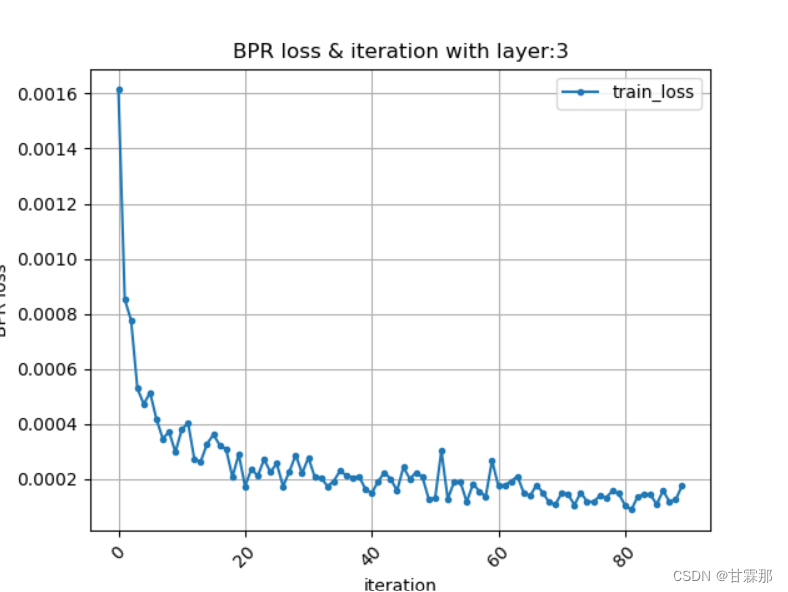
plt.figure()
plt.plot(x1[0:90], y4[0:90], '.-', label='train_loss')
plt.title('BPR loss & iteration with layer:3')
plt.ylabel('BPR loss')
plt.xlabel('iteration')
plt.xticks(rotation=45)
plt.legend()
plt.grid(True)
plt.savefig('MovieLens_BPR_loss_layer3.png')
plt.figure()
plt.plot(x1[0:90], y3[0:90], '.-', label='train_loss')
plt.title('BPR loss & iteration with layer:4')
plt.ylabel('BPR loss')
plt.xlabel('iteration')
plt.xticks(rotation=45)
plt.legend()
plt.grid(True)
plt.savefig('MovieLens_BPR_loss_layer4.png')
plt.figure()
plt.plot(x1[0:90], y5[0:90], '.-', label='train_loss')
plt.title('BPR loss & iteration with layer:3')
plt.ylabel('BPR loss')
plt.xlabel('iteration')
plt.xticks(rotation=45)
plt.legend()
plt.grid(True)
plt.savefig('yelp2018_BPR_loss_layer3.png')
plt.figure()
plt.plot(x1[0:90], y6[0:90], '.-', label='train_loss')
plt.title('BPR loss & iteration with layer:3')
plt.ylabel('BPR loss')
plt.xlabel('iteration')
plt.xticks(rotation=45)
plt.legend()
plt.grid(True)
plt.savefig('gowalla_BPR_loss_layer3.png')
pkl_file1.close()
pkl_file2.close()
pkl_file3.close()
pkl_file4.close()
pkl_file3_1.close()
pkl_file3_2.close()
plt.figure(figsize=(13, 4))
# 构造x轴刻度标签、数据
labels = [ 'yelp2018','MovieLens','gowalla']
first = [np.max(y5_1),np.max(y3_1),np.max(y6_1)]
second = [np.max(y5_2),np.max(y3_2),np.max(y6_2)]
third = [np.max(y5_3),np.max(y3_3),np.max(y6_3)]
plt.figure()
# 三组数据
x = np.arange(len(labels)) # x轴刻度标签位置
width = 0.2 # 柱子的宽度
# 计算每个柱子在x轴上的位置,保证x轴刻度标签居中
# x - width,x, x + width即每组数据在x轴上的位置
plt.bar(x - width, first, width, label='NDCG')
plt.bar(x, second, width, label='precision')
plt.bar(x + width, third, width, label='recall')
plt.ylabel('Scores')
plt.title('NDCG & precision & recall')
# x轴刻度标签位置不进行计算
plt.xticks(x, labels=labels)
plt.legend()
plt.savefig('different_dataset_compare.png')
plt.figure(figsize=(13, 4))
# 构造x轴刻度标签、数据
labels = ['layer1', 'layer2', 'layer3', 'layer4']
first = [np.max(y4_1),np.max(y3_1),np.max(y2_1),np.max(y1_1)]
second = [np.max(y4_2),np.max(y3_2),np.max(y2_2),np.max(y1_2)]
third = [np.max(y4_3),np.max(y3_3),np.max(y2_3),np.max(y1_3)]
plt.figure()
# 三组数据
x = np.arange(len(labels)) # x轴刻度标签位置
width = 0.2 # 柱子的宽度
# 计算每个柱子在x轴上的位置,保证x轴刻度标签居中
# x - width,x, x + width即每组数据在x轴上的位置
plt.bar(x - width, first, width, label='NDCG')
plt.bar(x, second, width, label='precision')
plt.bar(x + width, third, width, label='recall')
plt.ylabel('Scores')
plt.title('NDCG & precision & recall')
# x轴刻度标签位置不进行计算
plt.xticks(x, labels=labels)
plt.legend()
plt.savefig('different_layers_compare.png')
结果展示:(仅展示部分)