相关课程:【音频信号处理及深度学习教程】
0
信号的叠加:https://teropa.info/harmonics-explorer/
一个复杂信号分解成若干简单信号分量之和。不同个频率信号的叠加: 由于和差化积,会形成包络结构与精细结构。
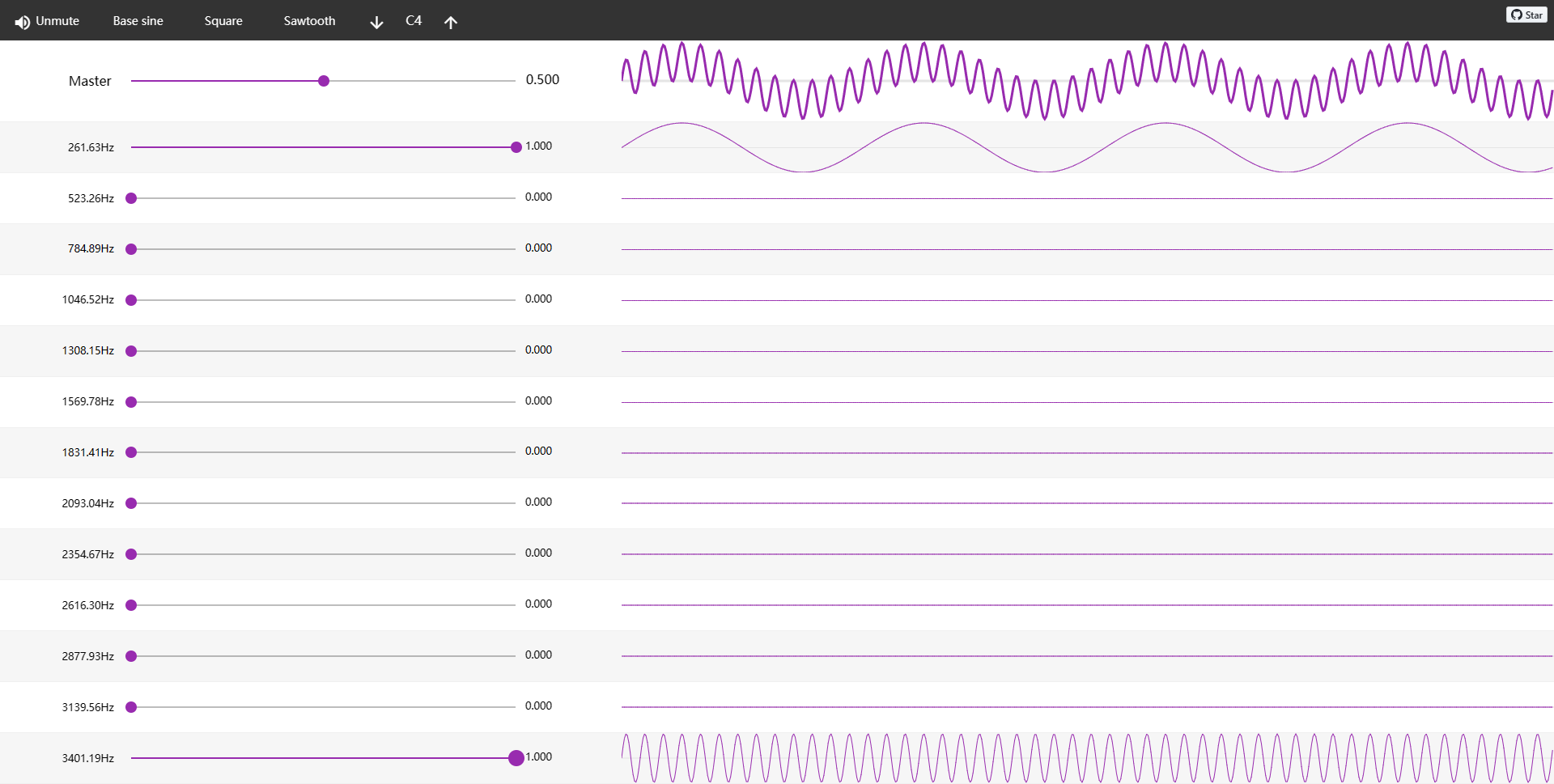
由上图可知,低频信号决定了信号的包络形状,高频信号决定其精细结构。
在语音识别中,主要通过信号的包络结构来区分不同音频信号,因此在识别领域更关注低频作用
1 信号的时域分析
1.1 分帧
分帧:将信号按照时间尺度分割,每一段的长度就是长frame_size,分出n段,为的个数frame_num,如果不考虑重叠分帧,那么该信号总的采样点数为frame_size * frame_n um。
分帧重叠:为了让分后的信号更加平滑,需要重叠分帧,也就是下一帧中包含上一帧的采样点,那么包含的点数就是重叠长度hop_size。
分帧补零:帧的个数frame_num= 总样本数N / 重叠数hop_size(分不补零),因为的个数frame_num是整数为了不舍弃最后一帧不能凑成一个完整长的点,需要对信号补零。此时帧的个数frame num =(总样本数N - 帧长frame size)/ 重叠数hop _size(分补零)+1
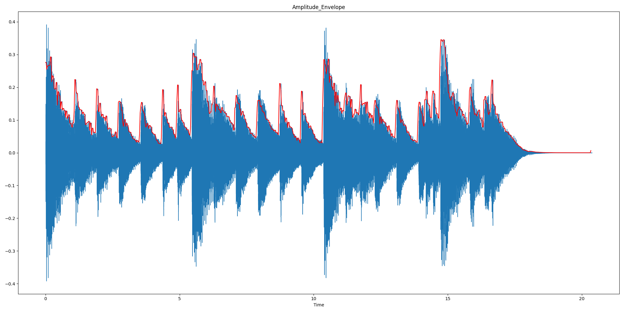
1.1.1 幅值包络
幅值包络:依次寻找每一帧的幅值最大值,将每一帧中幅值最大值连起来就是幅值包络(响度、音频检测、音频分类)
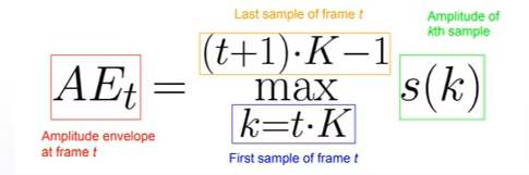
现提取第t帧的AE值,其中k是采样点数,t是序列数,K是每一帧的帧长,采样点k点在t k,(t+1) k-1
代码如下:
import librosa
import numpy as np
import librosa.display
from matplotlib import pyplot as plt
wave_path_absolute = r"E:\VoiceDev\audio_data\music_piano.wav"
wave_path = "../audio_data/music_piano.wav"
# 1. 加载信号以及采样率
waveform, sample_rate = librosa.load(wave_path_absolute, sr=None)
# 2. 定义AE函数,功能是取信号每一帧中幅值最值为该帧的包络
# 信号,每一帧长,重叠长度
def Calc_Amplitude_Envelope(waveform, frame_length, hop_length):
# 如果按照帧长来分割信号,余下部分不能形成一个帧则需要补0
if len(waveform) % hop_length != 0:
# ?
frame_num = int((len(waveform) - frame_length) / hop_length) + 1
pad_num = frame_num * hop_length + frame_length - len(waveform) # 补0个数
waveform = np.pad(waveform, pad_width=(0, pad_num), mode="wrap") # 补0操作
frame_num = int((len(waveform) - frame_length) / hop_length) + 1
waveform_ae = []
for t in range(frame_num):
current_frame = waveform[t * (frame_length - hop_length):t * (frame_length - hop_length) + frame_length]
current_ae = max(current_frame)
waveform_ae.append(current_ae)
return np.array(waveform_ae)
# 3. 设置参数:每一帧长1024,以50%的重叠率分帧,调用该函数
frame_size = 1024
hop_size = int(frame_size * 0.5)
waveform_AE = Calc_Amplitude_Envelope(waveform=waveform, frame_length=frame_size, hop_length=hop_size)
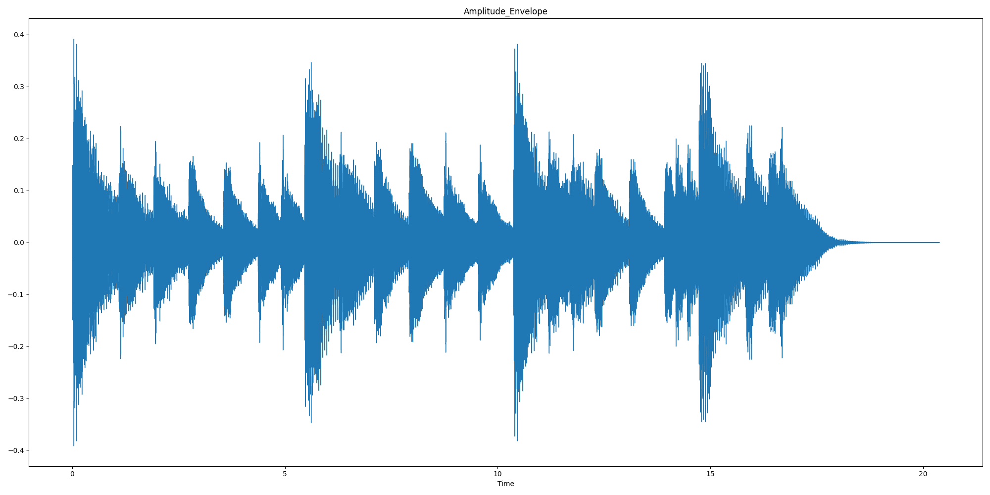
# 4.绘制信号的幅值包络信息
frame_scale = np.arange(0, len(waveform_AE))
time_scale = librosa.frames_to_time(frame_scale, hop_length=hop_size)
plt.figure(figsize=(20, 10))
librosa.display.waveshow(waveform)
plt.plot(time_scale, waveform_AE, color='red')
plt.title("Amplitude_Envelope")
plt.show()
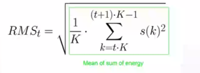
1.1.2 均方根能量
均方根能量(Root mean square energy)(响度、音频分段分类)
依次寻找每一帧中的RMSE,它的值为第t帧中每点幅值平方再取均值后开根号
代码如下:
# 0. 预设环境
import librosa
import numpy as np
from matplotlib import pyplot as plt
import librosa.display
# 1.加载信号
wave_path_absolute = r"E:\VoiceDev\audio_data\music_piano.wav"
wave_path = "../audio_data/music_piano.wav"
waveform, sample_rate = librosa.load(wave_path_absolute, sr=None)
# 2.定义函数RMS,功能:计算每一帧的均方根能量
def Calc_RMS(waveform, frame_length, hop_length):
# 如果按照帧长来分割信号,余下部分不能形成一个帧则需要补0
if len(waveform) % hop_length != 0:
# ?
frame_num = int((len(waveform) - frame_length) / hop_length) + 1
pad_num = frame_num * hop_length + frame_length - len(waveform) # 补0个数
waveform = np.pad(waveform, pad_width=(0, pad_num), mode="wrap") # 补0操作
frame_num = int((len(waveform) - frame_length) / hop_length) + 1
waveform_rms = []
for t in range(frame_num):
current_frame = waveform[t * (frame_length - hop_length):t * (frame_length - hop_length) + frame_length]
current_rms = np.sqrt(np.sum(current_frame**2) / frame_length)
waveform_rms.append(current_rms)
return waveform_rms
# 3. 设置参数:每一帧长1024,以50%的重叠率分帧,调用该函数
frame_size = 1024
hop_size = int(frame_size * 0.5)
waveform_RMS = Calc_RMS(waveform=waveform, frame_length=frame_size, hop_length=hop_size)
# 4.绘制图像
frame_scale = np.arange(0, len(waveform_RMS), step=1)
time_scale = librosa.frames_to_time(frame_scale, hop_length=hop_size)
plt.figure(figsize=(20, 10))
plt.plot(time_scale, waveform_RMS, color='red')
plt.title("Root-Mean-Square-Energy")
librosa.display.waveshow(waveform)
plt.show()
# 5. 利用librosa.feature.rms绘制信号的RMS
waveform_RMS_librosa = librosa.feature.rms(y=waveform, frame_length=frame_size, hop_length=hop_size).T[1:,0]
plt.figure(figsize=(20, 10))
plt.plot(time_scale, waveform_RMS_librosa, color='red')
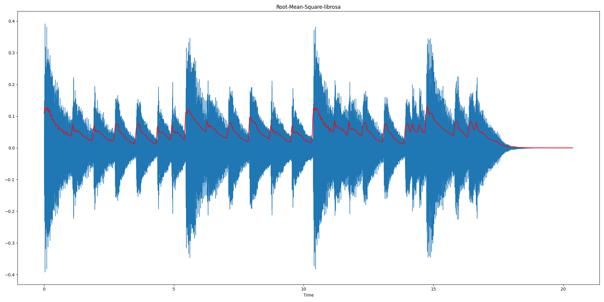
plt.title("Root-Mean-Square-librosa")
librosa.display.waveshow(waveform)
plt.show()
bias = waveform_RMS_librosa - waveform_RMS
print(f"the bias is {
bias}\n Congratulation!")
运行结果:红色线即均方根能量