一篇超超超长,超超超全面网络图绘制教程,本篇基本能讲清楚所有绘制要点,当然图论与网络优化的算法一篇不可能完全讲清楚,未来如果看的人多可以适当更新,同时做部分网络图绘图复刻。
以下是本篇绘图实验效果:


1 网络图创建
可以通过 graph 函数创建无向图,通过 digraph 创建有向图,其中网络创建可以使用起始终止点数组、邻接矩阵、EdgeTable等几种方式。
1.1 起始终止点数组
不点名布局时它会自动选择比较清晰的布局方式,怎么改布局之后再说,以下两个图连线情况都是一样的,不过有向图为了更好展示方向箭头自动用了不同的布局。
s=[1 1 1 1 1 1 1 9 9 9 9 9 9 9];
t=[2 3 4 5 6 7 8 2 3 4 5 6 7 8];
G=graph(s,t);
plot(G)

s=[1 1 1 1 1 1 1 9 9 9 9 9 9 9];
t=[2 3 4 5 6 7 8 2 3 4 5 6 7 8];
G=digraph(s,t);
plot(G)
1.2 邻接矩阵
无向图邻接矩阵必须是对称的,但是可以通过设置lower或upper属性使用下三角或上三角矩阵。
s=[1 1 1 1 1 1 1 9 9 9 9 9 9 9];
t=[2 3 4 5 6 7 8 2 3 4 5 6 7 8];
A=zeros(max(s));
for i=1:length(s)
    A(s(i),t(i))=1;
    A(t(i),s(i))=1;
end
% A = [0     1     1     1     1     1     1     1     0
%      1     0     0     0     0     0     0     0     1
%      1     0     0     0     0     0     0     0     1
%      1     0     0     0     0     0     0     0     1
%      1     0     0     0     0     0     0     0     1
%      1     0     0     0     0     0     0     0     1
%      1     0     0     0     0     0     0     0     1
%      1     0     0     0     0     0     0     0     1
%      0     1     1     1     1     1     1     1     0];
G=graph(A);
plot(G)
通过设置upper属性使用上三角矩阵:
s=[1 1 1 1 1 1 1 9 9 9 9 9 9 9];
t=[2 3 4 5 6 7 8 2 3 4 5 6 7 8];
A=zeros(max(s));
for i=1:length(s)
    A(min(s(i),t(i)),max(s(i),t(i)))=1;
end
% A = [0     1     1     1     1     1     1     1     0
%      0     0     0     0     0     0     0     0     1
%      0     0     0     0     0     0     0     0     1
%      0     0     0     0     0     0     0     0     1
%      0     0     0     0     0     0     0     0     1
%      0     0     0     0     0     0     0     0     1
%      0     0     0     0     0     0     0     0     1
%      0     0     0     0     0     0     0     0     1
%      0     0     0     0     0     0     0     0     0];
G=graph(A,'upper');
plot(G)
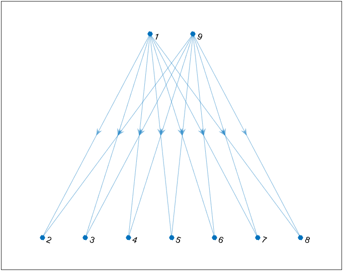
有向图第 i 行第 j 列有数值就说明有从 i 流向 j 的箭头。此处不要求对称矩阵啦。
s=[1 1 1 1 1 1 1 9 9 9 9 9 9 9];
t=[2 3 4 5 6 7 8 2 3 4 5 6 7 8];
A=zeros(max(s));
for i=1:length(s)
    A(s(i),t(i))=1;
end

G=digraph(A);
plot(G,'Layout','layered')

如果矩阵是对称的就说明流动是双向的:
s=[1 1 1 1 1 1 1 9 9 9 9 9 9 9];
t=[2 3 4 5 6 7 8 2 3 4 5 6 7 8];
A=zeros(max(s));
for i=1:length(s)
    A(s(i),t(i))=1;
    A(t(i),s(i))=1;
end

G=digraph(A);
plot(G,'Layout','layered')

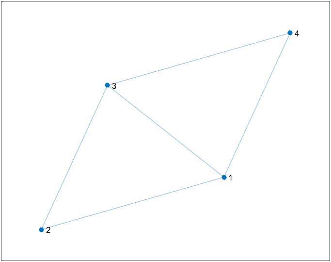
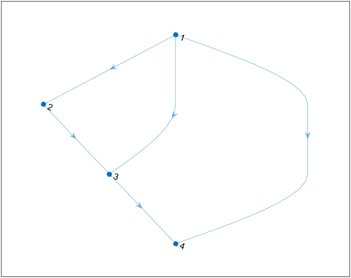
1.3 EdgeTable
先展示一下最简单的啥都没有的网络图,之后会给出边表中增添权重,增添标签名称啥的方法的!
s=[1 1 1 2 3];
t=[2 3 4 3 4];
EdgeTable=table([s' t'],'VariableNames',{

    'EndNodes'});
% EdgeTable =
%
%   5×1 table
%     EndNodes
%     ________
%      1    2
%      1    3
%      1    4
%      2    3
%      3    4
G=graph(EdgeTable);
plot(G)
s=[1 1 1 2 3];
t=[2 3 4 3 4];
EdgeTable=table([s' t'],'VariableNames',{

    'EndNodes'});
G=digraph(EdgeTable);
plot(G)
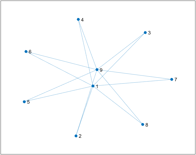
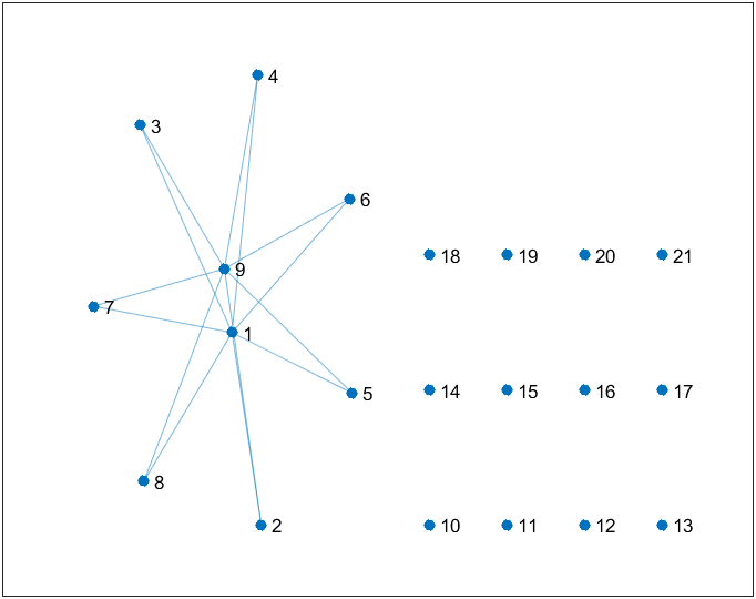
1.4 指定节点数量
通过如下方式可以设置节点总数:
s=[1 1 1 1 1 1 1 9 9 9 9 9 9 9];
t=[2 3 4 5 6 7 8 2 3 4 5 6 7 8];
G=graph(s,t,[],21);
plot(G)
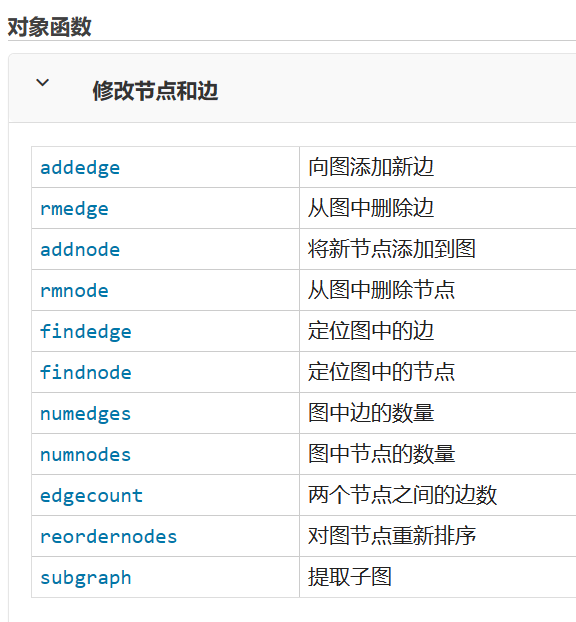
1.5 节点及边的增添
实际上是使用,以下的 addnode 及 addedge 函数实现的:
s=[1 1 1 1 1 1 1 9 9 9 9 9 9 9];
t=[2 3 4 5 6 7 8 2 3 4 5 6 7 8];
G=digraph(s,t);

G=G.addnode(5);
plot(G)

G=G.addedge(10,14);
plot(G)

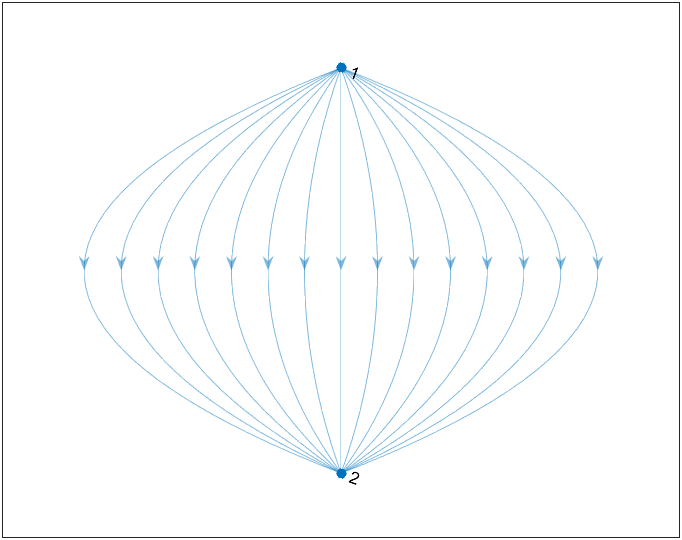
1.6 边数量说明
两点之间不仅仅只能有两条边。
s=ones(1,15);
t=2.*ones(1,15);
G=digraph(s,t);
plot(G)
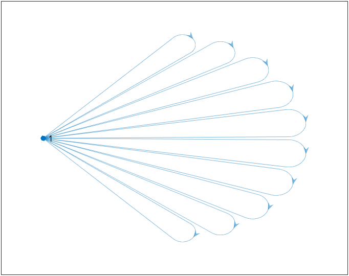
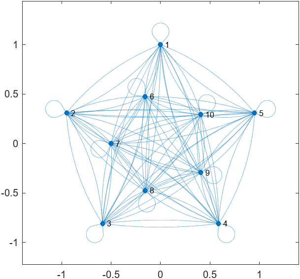
自己到自己的边也是可以有且能有很多条的:
s=ones(1,10);
t=ones(1,10);
G=digraph(s,t);
plot(G)
2 标签添加
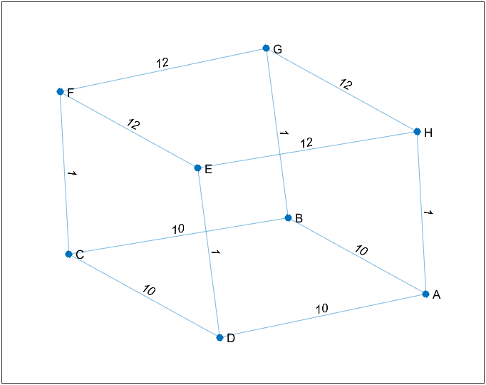
2.1 权重添加及节点命名
对于由起始终止点数组创建的图:
s=[1 1 1 2 2 3 3 4 5 5 6 7];
t=[2 4 8 3 7 4 6 5 6 8 7 8];
weights=[10 10 1 10 1 10 1 1 12 12 12 12];
names={

    'A' 'B' 'C' 'D' 'E' 'F' 'G' 'H'};
G=graph(s,t,weights,names);
plot(G,'EdgeLabel',weights)
对于边表创建时增添权重及节点名称:
s=[1 1 1 2 2 3 3 4 5 5 6 7];
t=[2 4 8 3 7 4 6 5 6 8 7 8];
weights=[10 10 1 10 1 10 1 1 12 12 12 12];
names={

    'A' 'B' 'C' 'D' 'E' 'F' 'G' 'H'};
EdgeTable=table([s' t'],weights','VariableNames',{

    'EndNodes' 'Weights'});
NodeTable=table(names','VariableNames',{

    'Name'});
% EdgeTable =
%
%   12×2 table
%     EndNodes    Weights
%     ________    _______
%      1    2       10
%      1    4       10
%      1    8        1
%     ...  ...     ...
%      6    7       12
%      7    8       12
G=graph(EdgeTable,NodeTable);
plot(G,'EdgeLabel',weights)
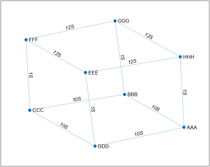
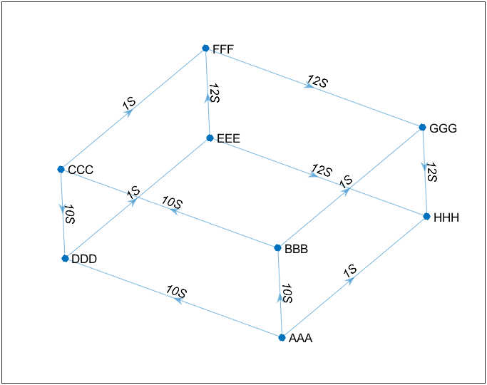
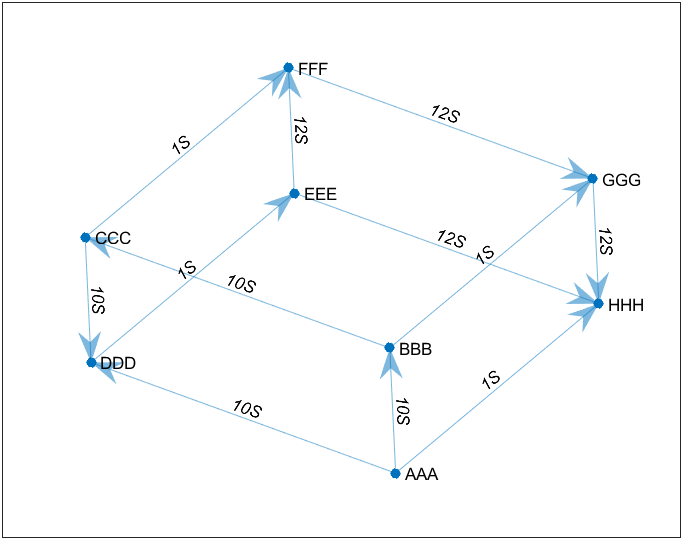
2.2 权重标签及节点标签修改
s=[1 1 1 2 2 3 3 4 5 5 6 7];
t=[2 4 8 3 7 4 6 5 6 8 7 8];
weights=[10 10 1 10 1 10 1 1 12 12 12 12];
names={

    'A' 'B' 'C' 'D' 'E' 'F' 'G' 'H'};
codeW={

    '10S','10S','1S','10S','1S','10S','1S','1S','12S','12S','12S','12S'};
codeN={

    'AAA' 'BBB' 'CCC' 'DDD' 'EEE' 'FFF' 'GGG' 'HHH'};
G=graph(s,t,weights,names);
plot(G,'EdgeLabel',codeW,'NodeLabel',codeN)
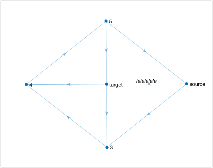
当然可以仅仅为部分添加:
s=[1 1 2 2 3 4 5 5];
t=[2 3 3 4 4 5 1 2];
G=digraph(s,t);
h=plot(G);
labelnode(h,[1 2],{

    'source' 'target'})
labeledge(h,1,2,'lalalalala')
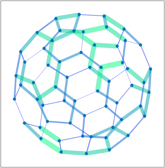
2.3 highlight
比如说把如下点和边标为红色:
G=digraph(bucky);
h=plot(G);

highlight(h,[8,7,6,1,2,3,4,5,54,55],'NodeColor','red','MarkerSize',5)
highlight(h,[8,7,6,1,2,3,4,5,54,55],'EdgeColor','red','LineWidth',3)

axis tight equal
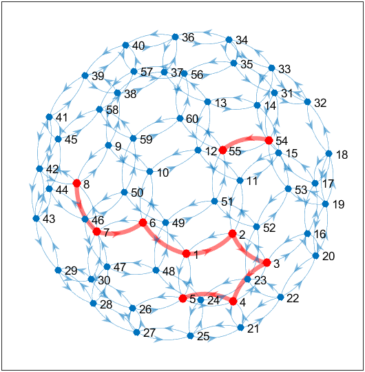
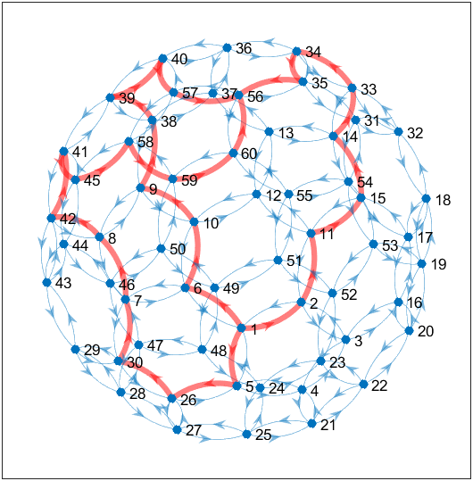
但其实最好用边表来增添高亮,很多图论与网络优化官方函数的返回值都是边表:
G=digraph(bucky);
h=plot(G);
[mf,GF]=maxflow(G,1,56);

highlight(h,GF,'EdgeColor','red','LineWidth',3)

axis tight equal
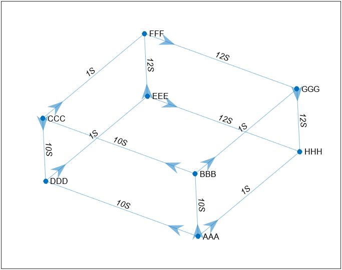
3 基础属性
以下操作在如下例子的基础上进行:
s=[1 1 1 2 2 3 3 4 5 5 6 7];
t=[2 4 8 3 7 4 6 5 6 8 7 8];
weights=[10 10 1 10 1 10 1 1 12 12 12 12];
names={

    'A' 'B' 'C' 'D' 'E' 'F' 'G' 'H'};
codeW={

    '10S','10S','1S','10S','1S','10S','1S','1S','12S','12S','12S','12S'};
codeN={

    'AAA' 'BBB' 'CCC' 'DDD' 'EEE' 'FFF' 'GGG' 'HHH'};
G=digraph(s,t,weights,names);
h=plot(G,'EdgeLabel',codeW,'NodeLabel',codeN,'Layout','subspace');
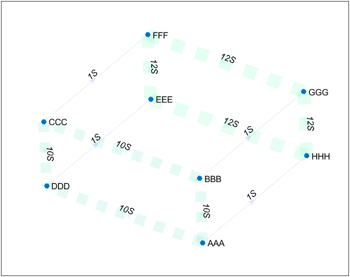
3.1 线条属性
线条粗细:
h.LineWidth=weights;

线条颜色:
h.EdgeColor=[0,0,0];

线条颜色映射:
h.EdgeCData=weights;
colormap(winter)

线条样式:
h.LineStyle=':';

透明度:
h.EdgeAlpha=.1;
3.2 节点属性
节点大小:
h.MarkerSize=(1:8).*3;

节点颜色:
h.NodeColor='red';%[1,0,0]
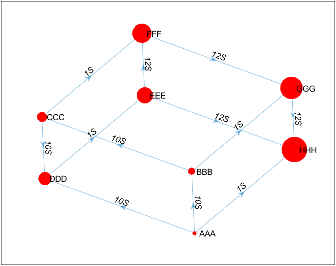
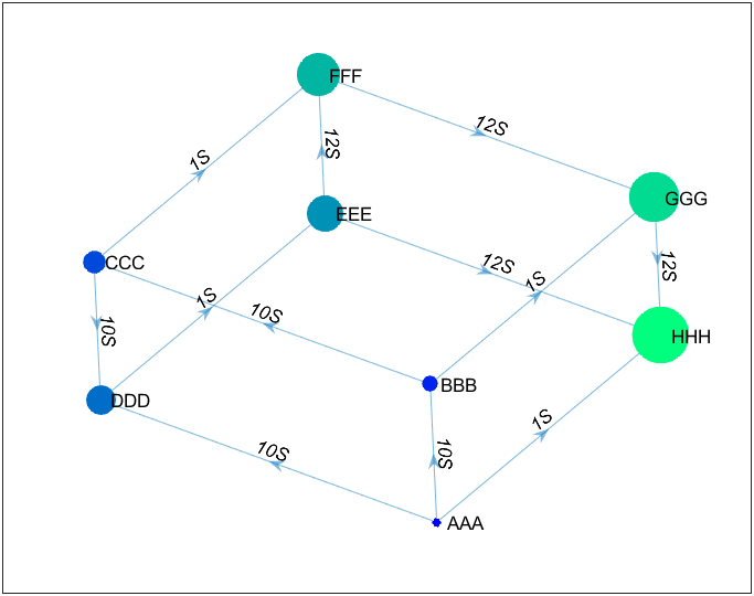
节点颜色映射:
h.NodeCData=1:8;
节点形状:
h.Marker="^";

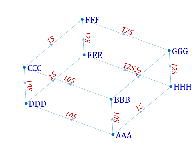
3.3 标签属性
标签各个属性名就加个Node或者Edge即可:
h.NodeFontName='Cambria';
h.NodeFontSize=15;
h.NodeLabelColor=[0,0,.8];

h.EdgeFontName='Cambria';
h.EdgeFontSize=13;
h.EdgeLabelColor=[.8,0,0];
3.4 箭头属性
箭头大小:
h.ArrowSize=15;
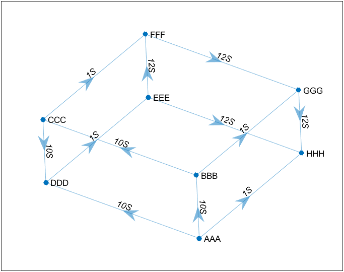
箭头位置,范围0-1比例,0时代表在末尾,1时代表在头部
h.ArrowPosition=1;
h.ArrowPosition=.2;
3.5 类比plot函数
老版本就可以像正常plot函数一样设置属性,属性设置可以写的比较随意,而且和普通plot含函数绘图非常类似,甚至这样都行:
G=graph(bucky);
plot(G,'-.dr','NodeLabel',{

    })
axis tight equal

G=graph(bucky);
G.Edges.Weight=rand(size(G.Edges.Weight));

plot(G,'NodeLabel',{

    },'EdgeCData',G.Edges.Weight,'LineWidth',G.Edges.Weight.*8)
colormap(winter)
axis tight equal
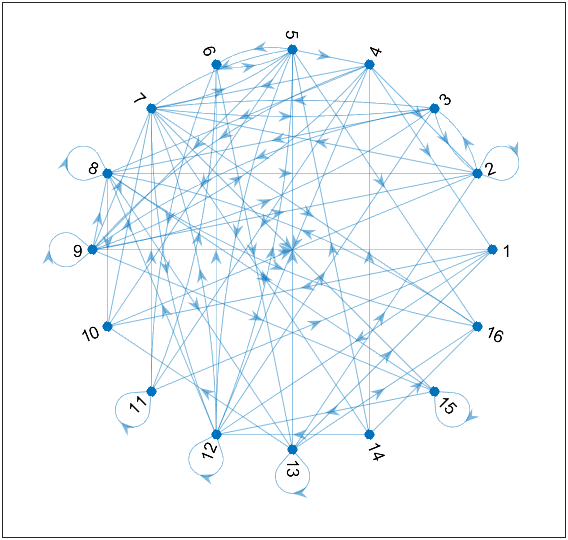
4 网络图布局
4.1 circle布局
就是节点均匀分布在圆上:
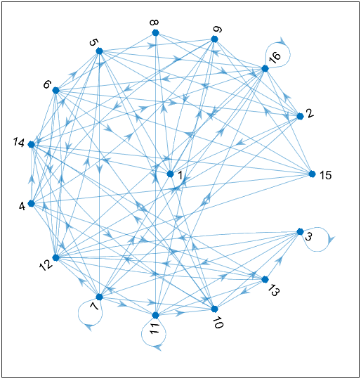
A=rand(16)>.7;
G=digraph(A);
plot(G,'Layout','circle')
axis tight equal
把节点1放在中央:
A=rand(16)>.7;
G=digraph(A);
plot(G,'Layout','circle','Center',1)
axis tight equal
4.2 force布局
在相邻节点之间使用引力,在远距离节点之间使用斥力:
s=[1 1 1 1 1 6 6 6 6 6 11 11 11];
t=[2 3 4 5 6 7 8 9 10 11 12 13 14];
G=graph(s,t);
plot(G,'Layout','force');
增添权重影响,权重越大的边越长:
s=[1 1 1 1 1 6 6 6 6 6 11 11 11];
t=[2 3 4 5 6 7 8 9 10 11 12 13 14];
weights=randi([1 20],1,13);

G=graph(s,t,weights);
plot(G,'Layout','force','WeightEffect','direct');
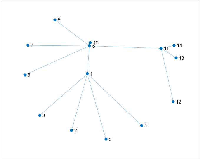
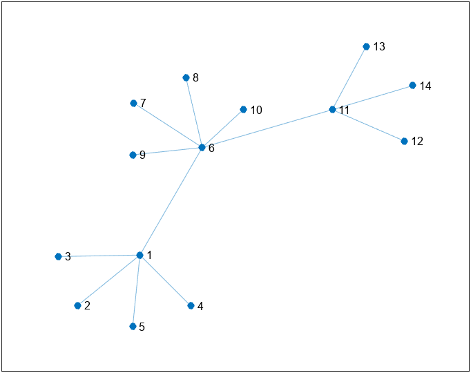
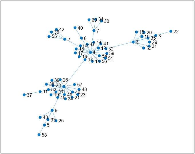
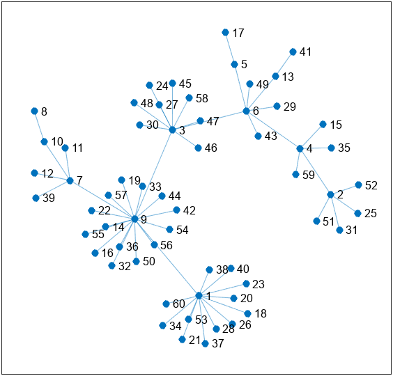
通过调整’Iterations’改变引力模拟迭代次数,以下举迭代10次和迭代1000次例子(迭代的初始X,Y坐标可通过’XStart’及’YStart’属性设置以保证每次实验结果相同,此处不再赘述):
% 随便生成一组最小生成树
A=rand(60)>.7;
G=graph(A,'upper');
T=minspantree(G);

plot(T,'Layout','force','Iterations',10);
plot(T,'Layout','force','Iterations',1000);
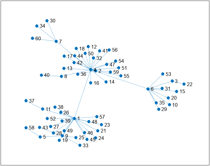
围绕原点:
% 随便生成一组最小生成树
A=rand(60)>.7;
G=graph(A,'upper');
T=minspantree(G);

plot(T,'Layout','force','UseGravity',true);
axis tight equal
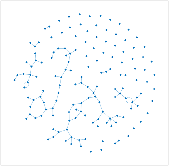
给个更直观的例子:
s=[1 3 5 7 7 10:100];
t=[2 4 6 8 9 randi([10 100],1,91)];
G=graph(s,t,[],150);

plot(G,'Layout','force','UseGravity',true);
axis tight equal
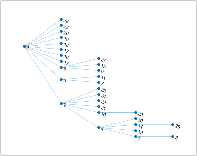
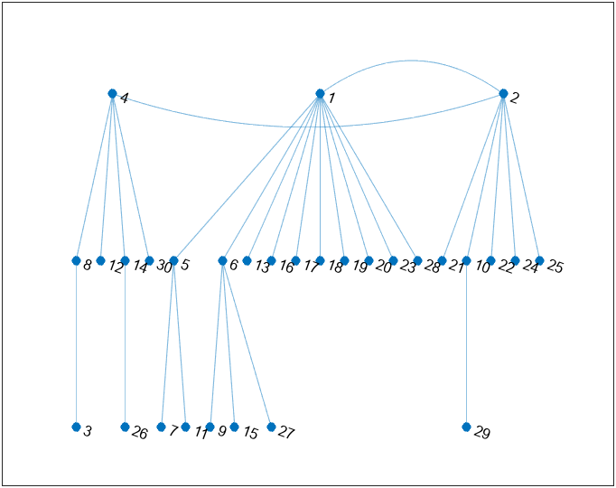
4.3 layered布局
有层次的树状布局:
% 随便生成一组最小生成树
A=rand(30)>.7;
G=graph(A,'upper');
T=minspantree(G)

plot(T,'Layout','layered')

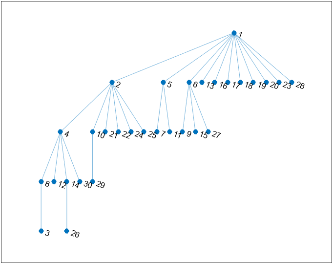
通过设置’Direction’ 设置方向,可选为’down’ | ‘up’ | ‘left’ | ‘right’
plot(T,'Layout','layered','Direction','right')
'Sources’属性可用来设置哪些点在第一层,'Sinks’属性可用来设置哪些点在最后一层:
plot(T,'Layout','layered','Sources',[1,2,4])
‘AssignLayers’属性可用来设置层分配方法,可选为’auto’ | ‘asap’ | ‘alap’
- auto: 节点分配使用 ‘asap’ 或 ‘alap’,以两者中更紧凑者为准。
- asap: 在分配节点时,在满足该节点所有前趋节点都必须在其之前的层的约束条件下,将其分配到尽可能靠前的层。
- alap: 在分配节点时,在满足其所有后继节点都必须在其之后的层的约束条件下,将其分配到尽可能后的层。
plot(T,'Layout','layered','AssignLayers','asap')
plot(T,'Layout','layered','AssignLayers','alap')

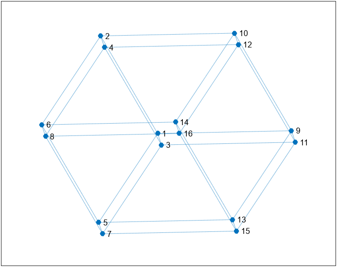
4.4 subspace布局
在高维嵌入式子空间中绘制图节点,然后将位置投影回二维。默认情况下,子空间维度是100或节点总数(以两者中较小者为准):
s=[1 1 1 2 2 3 3 4 5 5 6 7];
t=[2 4 8 3 7 4 6 5 6 8 7 8];

G=graph(s,t);
plot(G,'Layout','subspace');

通过’Dimension’设置高维空间维数。
XYZW=(abs(dec2bin(0:2^4-1))-48.5).*2;
IPT=tril(XYZW*(XYZW'));
[rows,cols]=find(IPT==2);

G=graph(rows,cols);
plot(G,'Layout','subspace');
plot(G,'Layout','subspace','Dimension',5)

4.5 force3布局
与force布局可设置属性几乎完全一样不过是三维的:
A=rand(30)>.7;
G=graph(A,'upper');
T=minspantree(G);

plot(T,'Layout','force3','UseGravity',true);
axis tight equal

4.6 subspace3布局
与subspace布局可设置属性几乎完全一样不过是三维的:
XYZW=(abs(dec2bin(0:2^4-1))-48.5).*2;
IPT=tril(XYZW*(XYZW'));
[rows,cols]=find(IPT==2);

G=graph(rows,cols);
plot(G,'Layout','subspace3','Dimension',13);

4.7 自定义X,Y坐标布局
弄个心形:
posXY=[-0.1598   -0.0682; 0.3117   -0.0060;-0.0389    0.4154;-0.1874    0.5155;
       -0.3877    0.5691;-0.6693    0.5397;-0.8092    0.2599;-0.7522   -0.0959;
       -0.5915   -0.3515;-0.4465   -0.5294;-0.2668   -0.6503;-0.0060   -0.7867;
        0.2202   -0.6503; 0.4275   -0.5173; 0.5933   -0.3515; 0.7228   -0.1563;
        0.8040    0.1045; 0.7642    0.3653; 0.5259    0.5622; 0.2323    0.5121];

A=ones(20)>0;
[s,t]=find(A);

G=graph(s,t);
plot(G,'XData',posXY(:,1),'YData',posXY(:,2))
A=ones(10)>0;
[s,t]=find(A);

T=linspace(0,2*pi,6);T(end)=[];
X=[cos(T+pi/2),cos(T+pi/2+pi/10).*.5];
Y=[sin(T+pi/2),sin(T+pi/2+pi/10).*.5];

G=graph(s,t);
plot(G,'XData',X,'YData',Y)
axis tight equal
5 修饰案例
其实也算是给出一些好看的绘图模板叭,喜欢看的人多以后可以单独出几期绘图复刻啥的。
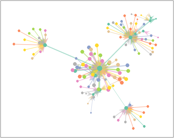
5.1 conncomp分类
s=[randi([1 50],1,40),randi([51 60],1,5),61:120];
t=[randi([1 50],1,40),randi([51 60],1,5),randi([61,120],1,60)];
G=graph(s,t,[],150);

% 分割,并将孤立点归为一类
bins=conncomp(G);
newBins=bins;
tb=tabulate(bins);
[~,ind]=sort(tb(:,2),'descend');
nV=tb(ind,1);
nS=tb(ind,2);
for i=1:length(ind)
    if nS(i)>1
        newBins(bins==nV(i))=i;
    else
        newBins(bins==nV(i))=0;
    end
end
newBins=newBins+1;
% 基础绘图
G=digraph(s,t,[],150);
h=plot(G,'Layout','force','UseGravity',true);
axis tight equal
% 属性修饰
h.NodeCData=newBins;
h.EdgeColor=[0,0,0];
h.EdgeAlpha=.3;
h.LineWidth=2;
h.MarkerSize=6+(newBins>1).*3;
CM=[0.4000    0.7608    0.6471
    0.9882    0.5529    0.3843
    0.5529    0.6275    0.7961
    0.9059    0.5412    0.7647
    0.6510    0.8471    0.3294
    1.0000    0.8510    0.1843
    0.8980    0.7686    0.5804
    0.7020    0.7020    0.7020];
CM=[CM;CM.*.6];
CM=[.8,.8,.8;CM];
colormap(CM(1:max(newBins),:))
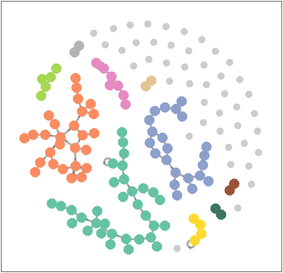
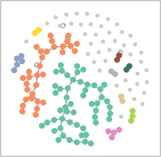
5.2 圆形网络图
% 先仅节点无边绘制带引力图记录X,Y坐标用于之后绘图
A=zeros(120);
G=digraph(A);
H=plot(G,'Layout','force','UseGravity',true);
X=H.XData;Y=H.YData;delete(H)
% 随机生成数据
A1=rand(20)>.92;
A2=rand(20)>.92;
A3=rand(20)>.92;
A5=zeros(20);
A=blkdiag(A1,A5,A2,A5,A3,A5);
[~,ind]=sort(rand(1,120));
A=A(ind,ind);
G=graph(A+A');
% 分割,并将孤立点归为一类
% 仅仅是示例,要有更好的分类算法或者早就分好类建议直接用
bins=conncomp(G);
newBins=bins;
tb=tabulate(bins);
[~,ind]=sort(tb(:,2),'descend');
nV=tb(ind,1);
nS=tb(ind,2);
for i=1:length(ind)
    if nS(i)>1
        newBins(bins==nV(i))=i;
    else
        newBins(bins==nV(i))=0;
    end
end
newBins=newBins+1;
% 绘图
G=digraph(A+A');
h=plot(G,'XData',X,'YData',Y);
axis tight equal
% 属性修饰
h.NodeCData=newBins;
h.EdgeCData=newBins(G.Edges.EndNodes(:,1));
h.EdgeAlpha=.4;
h.LineWidth=1;
h.MarkerSize=9;
CM=[0.4000    0.7608    0.6471
    0.9882    0.5529    0.3843
    0.5529    0.6275    0.7961
    0.9059    0.5412    0.7647
    0.6510    0.8471    0.3294
    1.0000    0.8510    0.1843
    0.8980    0.7686    0.5804
    0.7020    0.7020    0.7020];
CM=[CM;CM.*.6];
CM=[.8,.8,.8;CM];
colormap(CM(1:max(newBins),:))
set(gca,'XTick',[],'YTick',[])

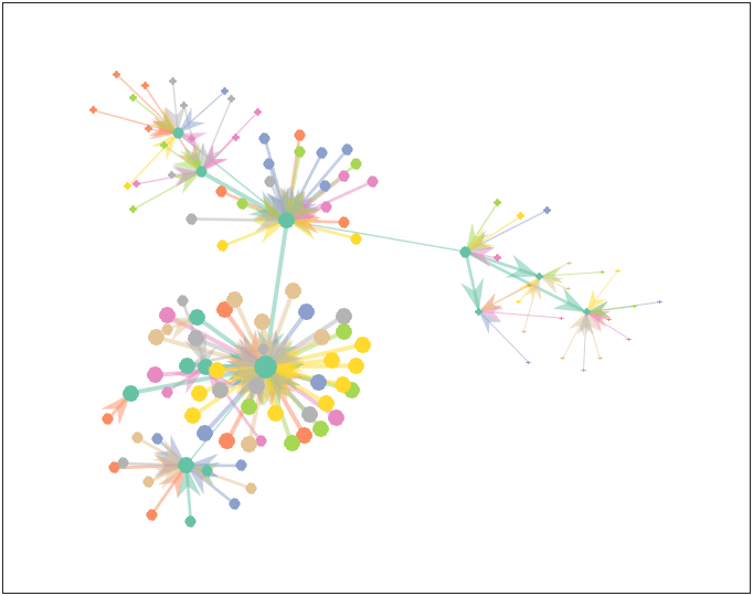
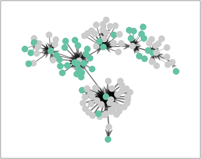
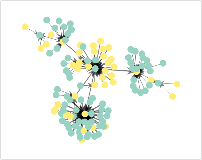
5.3 多彩的树状图
n=120;
A=rand(120)>.7;
G=graph(A,'upper');
T=minspantree(G,'Root',1);
L=zeros(1,n);
for i=1:n
    L(i)=length(shortestpath(T,1,i));
end
T=digraph(T.Edges.EndNodes(:,2),T.Edges.EndNodes(:,1));
% 基础绘图
h=plot(T,'Layout','force','Iterations',5);
h.MarkerSize=((max(L)-L)./max(L).*10./4+1).^2;
h.LineWidth=(max(L(2:end))-L(2:end))./max(L(2:end)).*3+.1;
h.ArrowSize=(max(L(2:end))-L(2:end))./max(L(2:end)).*10+10;
h.ArrowPosition=1;
% 设置配色
h.EdgeCData=T.Edges.EndNodes(:,1);
h.NodeCData=1:n;
CM=[0.4000    0.7608    0.6471
    0.9882    0.5529    0.3843
    0.5529    0.6275    0.7961
    0.9059    0.5412    0.7647
    0.6510    0.8471    0.3294
    1.0000    0.8510    0.1843
    0.8980    0.7686    0.5804
    0.7020    0.7020    0.7020];
colormap(CM)
修改一下配色:
n=120;
A=rand(120)>.7;
G=graph(A,'upper');
T=minspantree(G,'Root',1);
L=zeros(1,n);
for i=1:n
    L(i)=length(shortestpath(T,1,i));
end
T=digraph(T.Edges.EndNodes(:,2),T.Edges.EndNodes(:,1));
% 基础绘图
h=plot(T,'Layout','force','Iterations',5);
h.MarkerSize=10;
h.LineWidth=(max(L(2:end))-L(2:end))./max(L(2:end)).*3+.1;
h.ArrowSize=(max(L(2:end))-L(2:end))./max(L(2:end)).*10+10;
h.ArrowPosition=1;
% 设置配色
h.EdgeColor=[0,0,0];
h.NodeCData=mod(L,2)+1;
CM=[.8,.8,.8
    0.4000    0.7608    0.6471];
colormap(CM)

CM=[152,210,195
    254,237,119]./255;
colormap(CM)

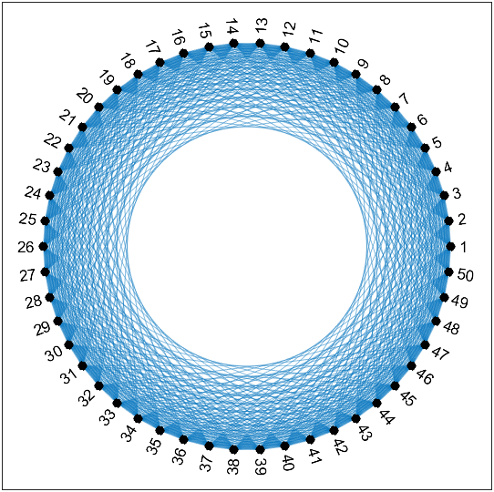
5.4 Watts-Strogatz 小世界图形
Watts-Strogatz 模型是一个包含小世界网络属性(例如集群和平均短路径长度)的随机图形。详细介绍请见:
https://ww2.mathworks.cn/help/matlab/math/build-watts-strogatz-small-world-graph-model.html
创建 Watts-Strogatz 图形包含以下两个基本步骤:
- 创建一个环形网格,其中包含 N N N 个平均出入度为 2 K 2K 2K 的节点。每个节点都与任一侧的 K K K 个最近邻点相连。
- 对于图中的每条边,重新连接概率为 β \beta β的目标节点。重新连接的边不能是重复或自环的。
执行第一步操作之后,图形将是一个完美的环形网格。因此当 β = 0 \beta=0 β=0时,不会重新连接任何边,并且该模型会返回一个环形网格。而如果 β = 1 \beta=1 β=1,则所有边都将重新连接,并且环形网格会变成随机图形。
文件 WattsStrogatz.m 对无向图实现该图算法。根据上面的算法说明,输入参数为 N、K 和 beta。
% Copyright 2015 The MathWorks, Inc.

function h = WattsStrogatz(N,K,beta)
% H = WattsStrogatz(N,K,beta) returns a Watts-Strogatz model graph with N
% nodes, N*K edges, mean node degree 2*K, and rewiring probability beta.
%
% beta = 0 is a ring lattice, and beta = 1 is a random graph.

% Connect each node to its K next and previous neighbors. This constructs
% indices for a ring lattice.
s = repelem((1:N)',1,K);
t = s + repmat(1:K,N,1);
t = mod(t-1,N)+1;

% Rewire the target node of each edge with probability beta
for source=1:N
    switchEdge = rand(K, 1) < beta;

    newTargets = rand(N, 1);
    newTargets(source) = 0;
    newTargets(s(t==source)) = 0;
    newTargets(t(source, ~switchEdge)) = 0;

    [~, ind] = sort(newTargets, 'descend');
    t(source, switchEdge) = ind(1:nnz(switchEdge));
end

h = graph(s,t);
end
构建图,并圆形布局,重新连接概率为0:
h=WattsStrogatz(50,15,0);
plot(h,'NodeColor','k','Layout','circle');
axis tight equal
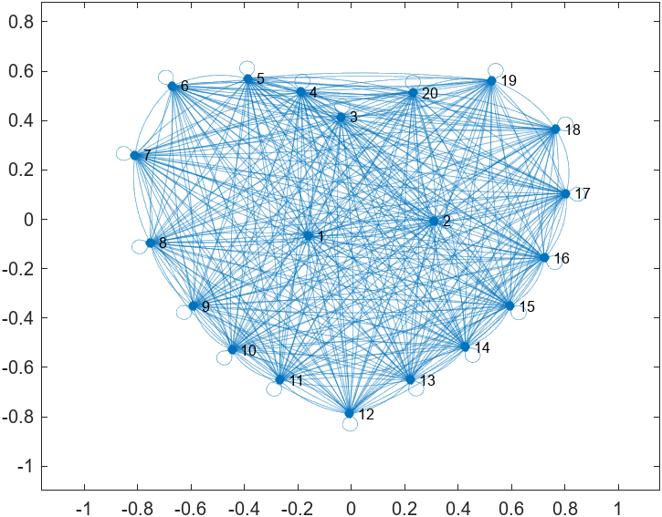
提高重新连接概率并计算出入度:
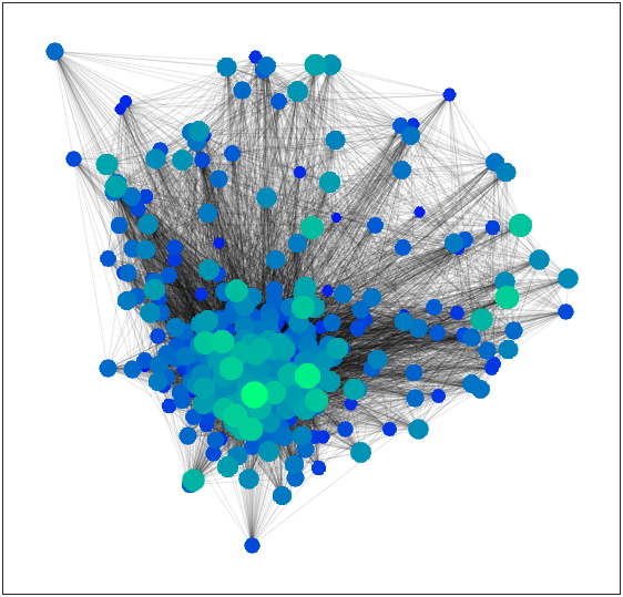
h2=WattsStrogatz(500,25,0.65);
H=plot(h2,'NodeColor','k','EdgeAlpha',0.1);
axis tight equal
H.EdgeColor=[0,0,0];
deg=degree(h2);
H.MarkerSize=2*sqrt(deg-min(deg)+0.2);
H.NodeCData=deg;
colormap(winter)


5.5 PageRank 算法对网站进行排名
又是官网的一个例子:
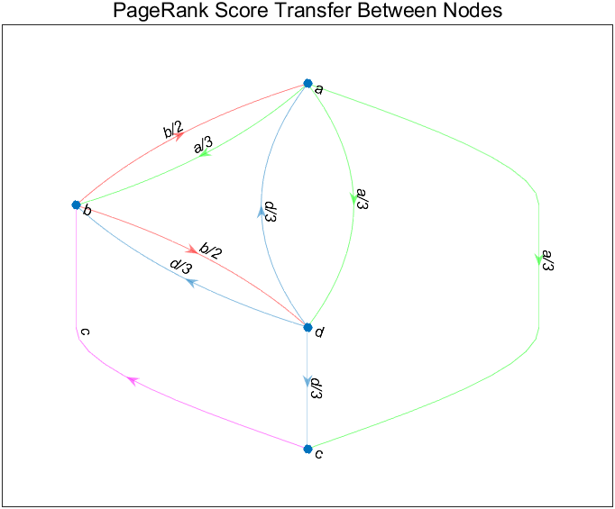
在 PageRank 算法的每一步中,每个网页的得分都会根据以下公式更新:
r = (1-P)/n + P*(A’*(r./d) + s/n)
- r 是 PageRank 得分的向量。
- P 是标量阻尼因子(通常为 0.85),这是随机浏览者点击当前网页上的链接而不是在另一随机网页上继续点击的概率。
- A’ 是图形的邻接矩阵的转置。
- d 是包含图形中每个节点的出度的向量。对于没有外向边的节点,d 设置为 1。
- n 是图形中节点的标量数量。
- s 是无链接的网页的 PageRank 得分的标量总和。
换言之,每个网页的排名很大程度上基于与之链接的网页的排名。项 A’*(r./d) 会挑选出链接到图形中每个节点的源节点的得分,而得分按这些源节点的出站链接总数进行归一化。这确保了 PageRank 得分的总和始终为 1。例如,如果节点 1 链接到节点 2、3 和 4,则它会在算法的每次迭代期间向其中的每一个节点传送 1/3 的 PageRank 得分。
s = {

    'a' 'a' 'a' 'b' 'b' 'c' 'd' 'd' 'd'};
t = {

    'b' 'c' 'd' 'd' 'a' 'b' 'c' 'a' 'b'};
G = digraph(s,t);
labels = {

    'a/3' 'a/3' 'a/3' 'b/2' 'b/2' 'c' 'd/3' 'd/3' 'd/3'};
p = plot(G,'Layout','layered','EdgeLabel',labels);
highlight(p,[1 1 1],[2 3 4],'EdgeColor','g')
highlight(p,[2 2],[1 4],'EdgeColor','r')
highlight(p,3,2,'EdgeColor','m')
title('PageRank Score Transfer Between Nodes')
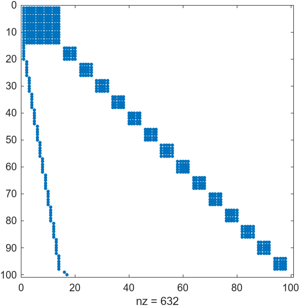
加载 mathworks100.mat 中的数据,并查看邻接矩阵 A。这些数据是使用自动网页趴chong程序在 2015 年生成的。网页趴chong程序从 https://www.mathworks.com 开始,然后是指向后续网页的链接,直到邻接矩阵包含 100 个唯一网页连接的相关信息。
load mathworks100.mat
spy(A)
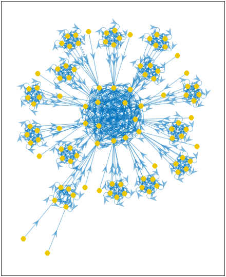
绘制网络图:
load mathworks100.mat
G=digraph(A,U);
plot(G,'NodeLabel',{

    },'NodeColor',[0.93 0.78 0],'Layout','force');
axis tight equal
MATLAB自带centrality函数可以计算重要性:
load mathworks100.mat
G=digraph(A,U);
pr = centrality(G,'pagerank','MaxIterations',200,'FollowProbability',0.85);
G.Nodes.PageRank = pr;
G.Nodes.InDegree = indegree(G);
G.Nodes.OutDegree = outdegree(G);

H=subgraph(G,find(G.Nodes.PageRank > 0.005));
h=plot(H,'NodeLabel',{

    },'NodeCData',H.Nodes.PageRank,'Layout','force');
colormap(parula(32))
colorbar
axis tight equal

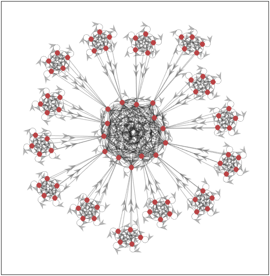
修改配色:
h.EdgeColor=[0,0,0];
h.EdgeAlpha=.3;
h.NodeColor=[185,67,69]./255;
colorbar('off')
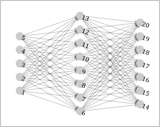
5.6 神经网络图
最多只能三层。三层往上建议自己写个函数。
layer=[5,8,7];
sumlayer=[0,cumsum(layer)];

S=[];T=[];
for i=1:length(layer)-1
    [tS,tT]=meshgrid(1:layer(i),1:layer(i+1));
    S=[S;tS(:)+sumlayer(i)];
    T=[T;tT(:)+sumlayer(i+1)];
end
G=digraph(S,T);
h=plot(G,'Layout','layered','Sources',1:layer(1),'AssignLayers','asap',...
    'Sinks',sumlayer(end-1)+1:sumlayer(end),'Direction','right');
h.ArrowPosition=1;
h.LineWidth=1;
h.EdgeColor=[0,0,0];
h.EdgeAlpha=.3;
h.ArrowSize=12;
h.MarkerSize=16;
h.NodeColor=[.8,.8,.8];
h.NodeFontSize=14;
h.NodeFontName='Cambria';
5.7 随便的一个树状图
E1=[ones(60,1),(2:61)'];
E2=[E1(randi([1,60],[90,1]),2),(62:151)'];
E3=[E2(randi([1,90],[150,1]),2),(152:301)'];
s=[E1(:,1);E2(:,1);E3(:,1)];
t=[E1(:,2);E2(:,2);E3(:,2)];
% 绘图
G=graph(s,t,t.*0+1);
h=plot(G,'Layout','force','WeightEffect','direct');
axis tight equal
% 修饰
h.EdgeColor=[0,0,0];
h.EdgeAlpha=.6;
h.MarkerSize=3;
h.NodeColor=[185,67,69]./255;

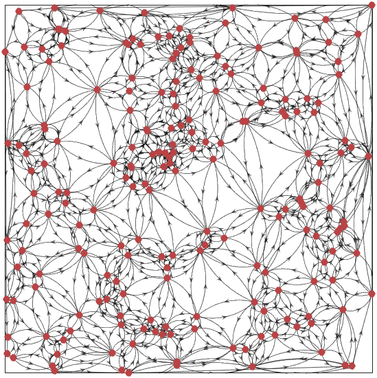
5.8 Delaunay 三角剖分
X=rand([200,1]);
Y=rand([200,1]);
% delaunay三角形生成
Tri=delaunay(X,Y);
S=[Tri(:,1);Tri(:,2);Tri(:,3)];
T=[Tri(:,2);Tri(:,3);Tri(:,1)];
% 绘图
G=digraph(S,T);
h=plot(G,'XData',X,'YData',Y);
% 修饰
axis equal
set(gca,'XLim',[0,1],'YLim',[0,1],'XTick',[],'YTick',[])
h.EdgeColor=[0,0,0];
h.EdgeAlpha=.6;
h.MarkerSize=4;
h.LineWidth=.5;
h.NodeColor=[185,67,69]./255;
完
又是一篇大长文结束
攒着想写的文章总算又干掉一篇
网络图绘制技能树get
编写不易希望大家多多点赞!!
全部代码mlx文件请以下gitee仓库获取: