1. 引言
前序博客有:
主要参考Justin Thaler 2022年8月在a16z crypto专题研讨会上的系列讲座:
SNARK方案由 Polynomial IOP ➕多项式承诺方案 组成。
当前的Polynomial IOP主要分为三大类:
- 1)基于interactive proofs(IPs)的Polynomial IOP:如Hyrax、vSQL、Libra、Virgo等。【 P P P无需做FFT运算】
- 2)基于multi-prover interactive proofs(MIPs)的Polynomial IOP:如Spartan、Brakedown、Xiphos等。【 P P P无需做FFT运算】
- 3)基于constant-round的Polynomial IOP:如Marlin、PlonK、StarkWare的SNARKs等。【 P P P需要做FFT运算】
以上方案都是通过增加 P P P开销,来减少proof长度以及降低 V V V开销。
以上1)2)类,只要其结合的多项式承诺方案也不需要FFT,则 P P P无需做FFT运算。
当前的多项式承诺方案主要分为四大类:
- 1)基于pairing的多项式承诺方案(既不transparent,也不post-quantum)
- 如KZG10、PST13、ZGKPP18等。
- 独特属性有:具有constant sized evaluation proofs。
- 2)基于discrete logarithm的多项式承诺方案(transparent,但不post-quantum)
- 如BCCGP16、Bulletproofs、Hyrax、Dory等。【其中Dory即需要discret-log hardness,还需要pairing。】
- 3)基于IOPs+hashing(transparent 且 post-quantum)
- 如Ligero、FRI、Brakedown等。
- 4)基于Groups of unknown order的多项式承诺方案(若使用class groups具有transparent属性,但不是post-quantum的)
- 如DARK、Dew等。
- 由于使用class groups, P P P非常慢。
本文将:
- 1)从“Multi-prover Interactive Proofs”(即基于MIP)的Polynomial IOP 分类中选择一个示例
- 2)从“IOPs+hashing”的多项式承诺方案 分类中选择一个示例
- 3)将以上1)2)2个示例组合,展示SNARK的工作原理
- 4)将以上1)2)2个示例组合,所构成的SNARK具有novel efficiency:
- 4.1)从文献来看,具有最快的 P P P(concretely and asymptotically);
- 4.2)可基于任意(足够大)的域(即具有field agnosticism(域不可知)属性);
- 4.3)首个实现见Brakedown [GLSTW21]:
- 详细见 Alexander Golovnev、Jonathan Lee、Srinath Setty、Justin Thaler和Riad S. Wahby等人2021年论文 Brakedown: Linear-time and post-quantum SNARKs for R1CS)
- 开源代码见:https://github.com/conroi/lcpc(Rust)
- 4.4)缺点在于:proof相当大——近期已对其进行了改进,可参看Tiancheng Xie等人2022年论文Orion: Zero Knowledge Proof with Linear Prover Time。【Orion改进了proof size,但是牺牲了field agnosticism(域不可知)属性。】

2. Polynomial IOP示例
本文的Polynomial IOP示例运行在Arithmetic Circuit Satisfiability上下文中。
所谓Arithmetic Circuit Satisfiability,是指:
- 已知某 arithmetic circuit C C C over F \mathbb{F} F of size S S S且输出为 y y y,判断是否存在某 w w w,使得 C ( w ) = y C(w)=y C(w)=y。
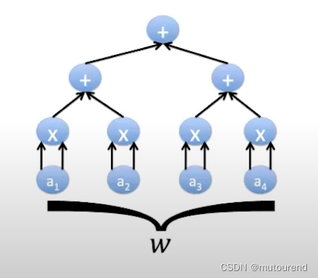
以 w = { a 1 , a 2 , a 3 , a 4 } , y = a 1 2 + a 2 2 + a 3 2 + a 4 2 w=\{a_1,a_2,a_3,a_4\}, y=a_1^2+a_2^2+a_3^2+a_4^2 w={
a1,a2,a3,a4},y=a12+a22+a32+a42为例:
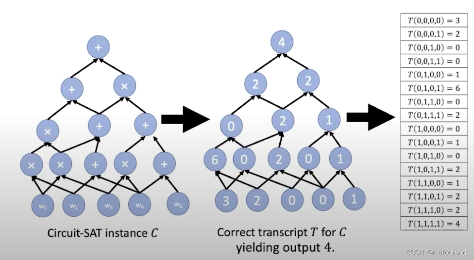
arithmetic circuit C C C 的 transcript T T T 是指:
- 对电路中每个gate的赋值
若电路中各个gate的赋值对应有效的witness w w w,则称 T T T为correct transcript。

可将transcript看成是 domain为 { 0 , 1 } log S \{0,1\}^{\log S} {
0,1}logS的function,为 C C C中的每个gate赋予 a ( log S ) − (\log S)- (logS)−bit gate label,看将 T T T看成是将gate labels映射为 F F F的函数:【逐层赋值】
所谓Polynomial IOP是指:
- 1) P P P的第一个message为某具有 ( log S ) (\log S) (logS)个变量的多项式 h h h, P P P声称该多变量多项式 h h h可extend a correct transcript T T T,即意味着:
h ( x ) = T ( x ) , ∀ x ∈ { 0 , 1 } log S h(x)=T(x),\forall x\in\{0,1\}^{\log S} h(x)=T(x),∀x∈{ 0,1}logS
仍以上图为例,相应的多变量多项式 h h h为:【可基于Boolean domain,借助multilinear Lagrange interpolation来获得多变量多项式】
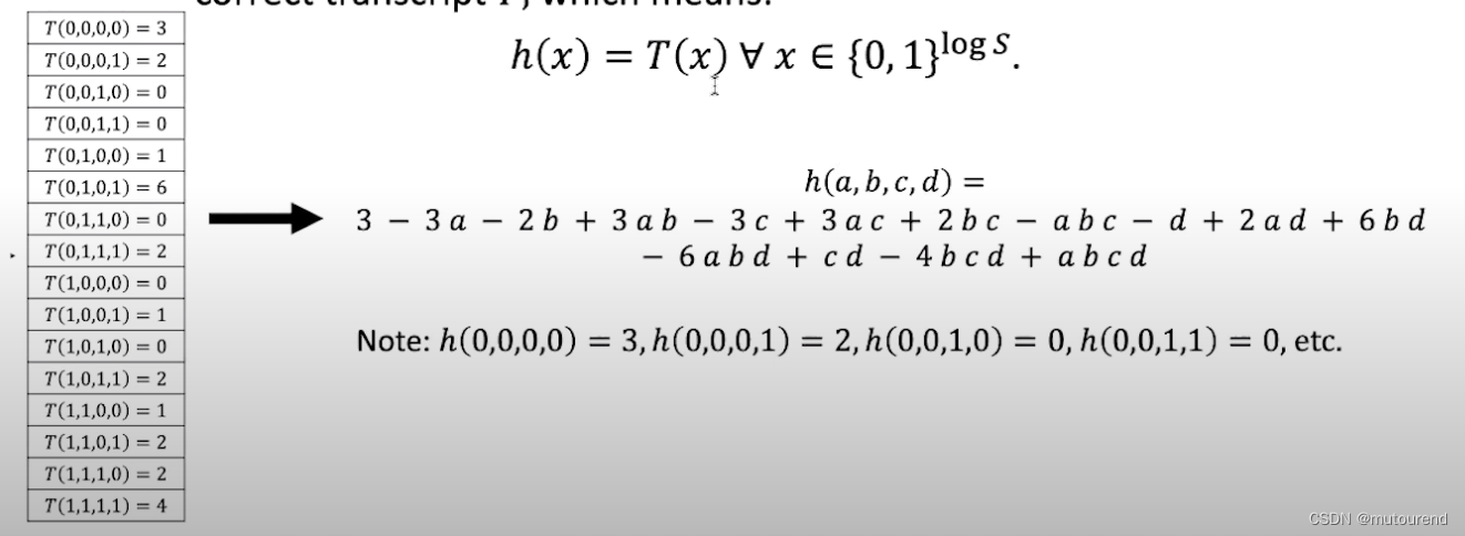
该多变量多项式 h h h满足: h ( 0 , 0 , 0 , 0 ) = 3 , h ( 0 , 0 , 0 , 1 ) = 2 , h ( 0 , 0 , 1 , 0 ) = 0 , h ( 0 , 0 , 1 , 1 ) = 0 h(0,0,0,0)=3,h(0,0,0,1)=2,h(0,0,1,0)=0,h(0,0,1,1)=0 h(0,0,0,0)=3,h(0,0,0,1)=2,h(0,0,1,0)=0,h(0,0,1,1)=0等等。
注意, h h h不仅适于 x ∈ { 0 , 1 } log S x\in\{0,1\}^{\log S} x∈{ 0,1}logS的情况,还适于所有 x ∈ F log S x\in \mathbb{F}^{\log S} x∈FlogS的情况:如, h ( 2 , 2 , 2 , 2 ) = − 19 h(2,2,2,2)=-19 h(2,2,2,2)=−19。
也就是说,transcript仅基于bit vectors域,而多变量多项式 h h h的定义域更大。 - 2) V V V需要检查 P P P声称的 h ( x ) = T ( x ) , ∀ x ∈ { 0 , 1 } log S h(x)=T(x),\forall x\in\{0,1\}^{\log S} h(x)=T(x),∀x∈{
0,1}logS成立,但是, V V V仅能learn a few evaluations of h h h。
为何 V V V仅凭少量evaluations of h h h,就可信服 P P P的声称呢?原因在于:- 2.1)将 h h h看成是对transcript T T T的distance-amplified encoding。
- 2.2) T T T的domain为 { 0 , 1 } log S \{0,1\}^{\log S} {
0,1}logS, h h h的domain为 F log S \mathbb{F}^{\log S} FlogS,要比 T T T的大得多。可称 h h h为 T T T的extension polynomial。
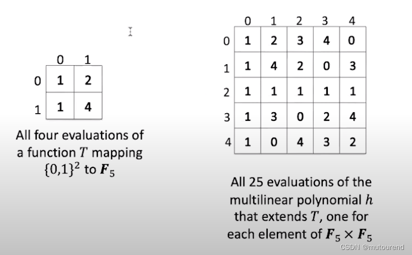
- 2.3)根据Schwartz-Zippel:若2个transcript T 和 T ′ T和T' T和T′哪怕仅有一个gate value值不同,二者相应的extension polynomial h 和 h ′ h和h' h和h′在 F log S \mathbb{F}^{\log S} FlogS内几乎所有的evaluation值都不相同(准确来说,不相同的概率为 1 − log ( S ) / ∣ F ∣ 1-\log (S)/|\mathbb{F}| 1−log(S)/∣F∣)。
- 2.4)这种encoding的distance-amplifying特性,使得,哪怕整个transcript中仅有一个“inconsistency”, V V V也可以发现。
Two-step plan of attack:
-
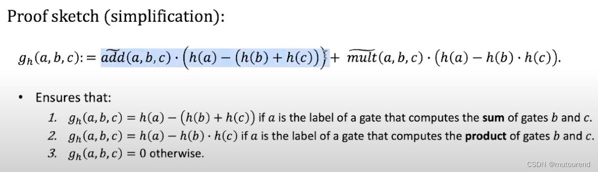
Step-1: 已知任意的 ( log S ) (\log S) (logS)个变量的多项式 h h h,找到相应的具有 ( 3 log S ) (3\log S) (3logS)个变量的多项式 g h g_h gh,使得:【可将 g h g_h gh看成是 h h h的ultra distance-amplified encoding。】
- h h h extends a correct transcript T T T,当且仅当,对于任意的 ∀ ( a , b , c ) ∈ { 0 , 1 } 3 log S \forall(a,b,c)\in\{0,1\}^{3\log S} ∀(a,b,c)∈{ 0,1}3logS,有 g h ( a , b , c ) = 0 g_h(a,b,c)=0 gh(a,b,c)=0。【即 g h g_h gh vanish over the Boolean hypercube,等价为, P P P的原始声称——即“ h h h extends a correct transcript T T T”。】
- 此外,为evaluate g h ( r ) g_h(r) gh(r) at any input r r r,足以通过evaluate h h h at only 3 inputs来实现。
为简化描述,以仅有乘法门的电路为例,可仅关注下述等式右侧的第二项,其输入为3个gate labels a , b , c a,b,c a,b,c,其中 m u l t ~ ( a , b , c ) \widetilde{mult}(a,b,c) mult (a,b,c)表示的是gates之间的wiring关系,也称为wiring polynomial。
-
Step-2: 为检查 g h ( a , b , c ) = 0 , ∀ ( a , b , c ) ∈ { 0 , 1 } 3 log S g_h(a,b,c)=0,\forall(a,b,c)\in\{0,1\}^{3\log S} gh(a,b,c)=0,∀(a,b,c)∈{ 0,1}3logS,设计了一个interactive proof:
- 其中 V V V仅需要evaluate g h ( r ) g_h(r) gh(r) at a single point r r r。
核心思路为:
-
1)先将 g h g_h gh想象为单变量多项式 g h ( X ) g_h(X) gh(X):
- 不同于,检查 g h g_h gh vanishes over input set { 0 , 1 } 3 log S \{0,1\}^{3\log S} { 0,1}3logS,转为,检查 g h g_h gh vanishes over some set H ⊆ F H\subseteq \mathbb{F} H⊆F。
-
2)事实上, g h ( x ) = 0 g_h(x)=0 gh(x)=0 for all x ∈ H x\in H x∈H,等价为, g h g_h gh可被 Z H ( x ) = ∏ a ∈ H ( x − a ) Z_H(x)=\prod_{a\in H}(x-a) ZH(x)=∏a∈H(x−a)整除。其中 Z H Z_H ZH称为the vanishing polynomial for H H H。
-
3)相应的Polynomial IOP为:
- 3.1) P P P发送多项式 q q q, q q q满足 g h ( X ) = q ( X ) ⋅ Z H ( X ) g_h(X)=q(X)\cdot Z_H(X) gh(X)=q(X)⋅ZH(X)。
- 3.2) V V V选择随机值 r ∈ F r\in \mathbb{F} r∈F,检查 g h ( r ) = q ( r ) ⋅ Z H ( r ) g_h(r)=q(r)\cdot Z_H(r) gh(r)=q(r)⋅ZH(r)是否成立。
- 3.2.1)事实上,若 H H H为 F \mathbb{F} F的additive subgroup或multiplicative subgroup,则 V V V计算 Z H ( r ) Z_H(r) ZH(r)的time为 O ( log ∣ H ∣ ) O(\log {|H|}) O(log∣H∣)。如,若 H H H为all n − n- n−roots of unity,则有 Z H ( r ) = r n − 1 Z_H(r)=r^n-1 ZH(r)=rn−1。
- 3.2.2)evaluate g h ( r ) g_h(r) gh(r) 需要 evaluate h h h at 3 3 3 points,而 q ( r ) q(r) q(r)则仅为one evaluation of q q q。
但是呢,现实情况是:
- (1) g h g_h gh不是单变量多项式,其具有 3 log S 3\log S 3logS个变量。且
- (2) P P P find and send quotient多项式 q q q是昂贵的:
- 在最终的SNARK中,意味着需为额外的多项式进行多项式承诺。
- 这是Marlin、PlonK、Groth16的实现方式,这也是为什么Marlin、PlonK、Groth16的Prover更慢的原因。
相应的解决方案为:使用sum-check protocol [LFKN90](即对应Lund等人1992年论文《Algebraic Methods for Interactive Proof Systems》):
- 可处理多变量多项式。
- 不要求 P P P发送额外的large polynomials。
事实上,为检查 g h ( a , b , c ) = 0 , ∀ ( a , b , c ) ∈ { 0 , 1 } 3 log S g_h(a,b,c)=0,\forall(a,b,c)\in\{0,1\}^{3\log S} gh(a,b,c)=0,∀(a,b,c)∈{ 0,1}3logS:
- (a) V V V会与 P P P一起运行sum-check protocol来计算:
∑ a , b , c ∈ { 0 , 1 } log S g h ( a , b , c ) 2 \sum_{a,b,c\in\{0,1\}^{\log S}}g_h(a,b,c)^2 ∑a,b,c∈{ 0,1}logSgh(a,b,c)2- 若该sum中所有项均为0,则最终的总和也为0;
- 若基于整数,该sum中的任意非零项,将导致最终的总和为strictly positive。
- (b)在sum-check protocol的结尾, V V V需要evaluate g h ( r 1 , r 2 , r 3 ) g_h(r_1,r_2,r_3) gh(r1,r2,r3)——为此,仅需要evaluate h ( r 1 ) 、 h ( r 2 ) 、 h ( r 3 ) h(r_1)、h(r_2)、h(r_3) h(r1)、h(r2)、h(r3)就足以。
Brakedown之前的SNARK方案:
避免FFT运算的原因如下3个:
- 1)若想要Prover尽可能快,应避免Prover做FFT运算,FFT运算的开销为 O ( n log n ) O(n\log n) O(nlogn),是super linear的。其中 n n n为circuit size。
- 2)避免FFT的另一个原因在于,仅有某些FFT-friendly域支持做FFT运算。
- 3)FFT运算不易并行化和distribute,通常硬件加速的瓶颈不在于computational bound,而在于memory bound。
附录A——sum-check protocol
可参考博客有:

附录B——Orion与Brakedown对比
Orion与Brakedown的多项式承诺方案性能对比:

注意,Brakedown的多项式承诺方案可用于任意域,而Orion的需要FFT-friendly域。
Orion与Brakedown等基于R1CS实现的zero-knowledge arguement对比:
