分割数据集为训练集，测试集及验证集的R实现

Using ‘splitTools’ (r-project.org)

介绍

splitTools是一种快速、便捷的数据分割方法，主要分为partition和create_folds两部分组成 .

数据分割(e.g. 分为训练集、测试集和验证集),
为交叉验证创建分割文件
为交叉验证创建重复文件
分层分割
组别分割，用于K折验证
分块分割（如果应该保留数据的顺序）

函数create_timefolds可以进行时间序列的分割，其中样本外的数据跟随（不断增长的）样本内数据。

现在我们将说明如何在一个典型的建模工作流程中使用splitTools。

数据分割

我们将进行一下三个步骤：

将iris数据集分成60%的训练数据、20%的验证数据和20%的测试数据，通过Sepal.Length这个变量进行分层。由于它是数字型的，所以内部通过量化分层来完成分层。
然后我们调整随机森林的参数mtry，以尽可能好地通过其他变量预测Sepal.Length。我们在验证数据上这样做。
选择最优mtry之后，在剩余的测试集上测试模型。

library(splitTools)
library(ranger)

# Split data into partitions
set.seed(3451)
inds <- partition(iris$Sepal.Length, p = c(train = 0.6, valid = 0.2, test = 0.2))
str(inds)
#> List of 3
#>  $ train: int [1:81] 2 3 6 7 8 10 11 18 19 20 ...
#>  $ valid: int [1:34] 1 12 14 15 27 34 36 38 42 48 ...
#>  $ test : int [1:35] 4 5 9 13 16 17 25 39 41 45 ...

train <- iris[inds$train, ]
valid <- iris[inds$valid, ]
test <- iris[inds$test, ]

# Root-mean-squared error function used to evaluate results
rmse <- function(y, pred) {
  sqrt(mean((y - pred)^2))
}

# Tune mtry on validation data
valid_mtry <- numeric(ncol(train) - 1)

for (i in seq_along(valid_mtry)) {
  fit <- ranger(Sepal.Length ~ ., data = train, mtry = i)
  valid_mtry[i] <- rmse(valid$Sepal.Length, predict(fit, valid)$predictions)
}

valid_mtry
#> [1] 0.3809234 0.3242173 0.3208119 0.3241518
(best_mtry <- which.min(valid_mtry))
#> [1] 3

# Fit and test final model
final_fit <- ranger(Sepal.Length ~ ., data = train, mtry = best_mtry)
rmse(test$Sepal.Length, predict(final_fit, test)$predictions)
#> [1] 0.3480947

交叉验证

由于我们的数据集只有150行，投入20%的观测值进行验证，既不稳健，也没有数据效率。让我们修改一下建模策略，用五倍交叉验证代替简单验证，再次使用响应变量的分层。

将鸢尾花的数据集分成80%的训练数据和20%的测试数据，按Sepal.Length这个变量分层。
在训练集上使用分层的五倍交叉验证法来调整参数mtry。
在通过这个简单的 "GridSearchCV "选择了最佳的mtry之后，我们在测试数据集上挑战最终的模型。

# Split into training and test
inds <- partition(iris$Sepal.Length, p = c(train = 0.8, test = 0.2))

train <- iris[inds$train, ]
test <- iris[inds$test, ]

# Get stratified cross-validation fold indices
folds <- create_folds(train$Sepal.Length, k = 5)

# Tune mtry by GridSearchCV
valid_mtry <- numeric(ncol(train) - 1)

for (i in seq_along(valid_mtry)) {
  cv_mtry <- numeric()
  for (fold in folds) {
    fit <- ranger(Sepal.Length ~ ., data = train[fold, ], mtry = i)
    cv_mtry <- c(cv_mtry, 
                 rmse(train[-fold, "Sepal.Length"], predict(fit, train[-fold, ])$predictions))
  }
  valid_mtry[i] <- mean(cv_mtry)
}

# Result of cross-validation
valid_mtry
#> [1] 0.3870915 0.3460605 0.3337763 0.3302831
(best_mtry <- which.min(valid_mtry))
#> [1] 4

# Use optimal mtry to make model
final_fit <- ranger(Sepal.Length ~ ., data = train, mtry = best_mtry)
rmse(test$Sepal.Length, predict(final_fit, test)$predictions)
#> [1] 0.2970876

重复交叉验证

如果可行的话，建议反复进行交叉验证，以减少决策的不确定性。这个过程和上面一样。我们不是在每个折中得到五个性能值，而是得到五倍的重复次数（这里是三个）。

# We start by making repeated, stratified cross-validation folds
folds <- create_folds(train$Sepal.Length, k = 5, m_rep = 3)
length(folds)
#> [1] 15

for (i in seq_along(valid_mtry)) {
  cv_mtry <- numeric()
  for (fold in folds) {
    fit <- ranger(Sepal.Length ~ ., data = train[fold, ], mtry = i)
    cv_mtry <- c(cv_mtry, 
                 rmse(train[-fold, "Sepal.Length"], predict(fit, train[-fold, ])$predictions))
  }
  valid_mtry[i] <- mean(cv_mtry)
}

# Result of cross-validation
valid_mtry
#> [1] 0.3934294 0.3544207 0.3422013 0.3393454
(best_mtry <- which.min(valid_mtry))
#> [1] 4

# Use optimal mtry to make model
final_fit <- ranger(Sepal.Length ~ ., data = train, mtry = best_mtry)
rmse(test$Sepal.Length, predict(final_fit, test)$predictions)
#> [1] 0.2937055

时间序列交叉验证和区块划分

当用时间序列数据建模时，使用交叉验证可能回破坏数据的时序属性，这种情况可以使用以下的交叉验证方法避免：

The data is first split into k+1k+1 blocks B1,...,Bk+1B1,...,Bk+1, in sequential order. Depending of type = "extending" (default) or type == "moving", the following data sets are used in cross-validation:

数据首先被分割成k+1块B1,...,Bk+1，按顺序排列。根据type="extending"（默认）或type=="moving"，以下数据集被用于交叉验证。

第一折: B1用来训练，B2用来验证
第二折:如果类型为 "extending"或 "moving"，B2用于训练，B3用于评估。
…
第K折: {B1,...,Bk} resp. 如果类型为 "extending"或 "moving"，Bk用于训练，Bk+1用于评估。

这些模式保证了评估数据集总是跟随训练数据。请注意，训练数据在整个过程中线性增长，类型="扩展"，而其长度在类型="移动 "时大致恒定。

为了对优化后的模型进行最终的评估，通常要做一个初始的封锁分割成连续的训练和测试数据。

例子

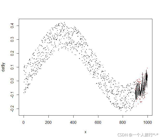
我们首先创建一个时间序列，并得出滞后的特征用于训练。然后，我们再次通过时间序列交叉验证来优化随机森林的mtry。我们在时间序列的最后10%上评估优化后的模型。

# Create data
set.seed(452)
n <- 1000
t <- seq(0, 2 * pi, length.out = n)
y <- 0.2 * sin(t) - 0.1 * cos(t) + 0.2 * runif(n)
plot(y ~ t, pch = ".", cex = 2)


# Helper function
Lag <- function(z, k = 1) {
  c(z[-seq_len(k)], rep(NA, k))
}
Lag(1:4, k = 1)
#> [1]  2  3  4 NA

# Add lagged features
dat <- data.frame(y, 
                  lag1 = Lag(y), 
                  lag2 = Lag(y, k = 2), 
                  lag3 = Lag(y, k = 3))
dat <- dat[complete.cases(dat), ]
head(dat)
#>              y         lag1         lag2        lag3
#> 1 -0.085447174  0.075314649 -0.007841658  0.10081516
#> 2  0.075314649 -0.007841658  0.100815165  0.09635395
#> 3 -0.007841658  0.100815165  0.096353945 -0.06476294
#> 4  0.100815165  0.096353945 -0.064762935  0.10474890
#> 5  0.096353945 -0.064762935  0.104748904  0.07030228
#> 6 -0.064762935  0.104748904  0.070302283  0.01085425
cor(dat)
#>              y      lag1      lag2      lag3
#> y    1.0000000 0.8789100 0.8858208 0.8840929
#> lag1 0.8789100 1.0000000 0.8791226 0.8858995
#> lag2 0.8858208 0.8791226 1.0000000 0.8791388
#> lag3 0.8840929 0.8858995 0.8791388 1.0000000

# Block partitioning
inds <- partition(dat$y, p = c(train = 0.9, test = 0.1), type = "blocked")
str(inds)
#> List of 2
#>  $ train: int [1:898] 1 2 3 4 5 6 7 8 9 10 ...
#>  $ test : int [1:99] 899 900 901 902 903 904 905 906 907 908 ...

train <- dat[inds$train, ]
test <- dat[inds$test, ]

# Get time series folds
folds <- create_timefolds(train$y, k = 5)
str(folds)
#> List of 5
#>  $ Fold1:List of 2
#>   ..$ insample : int [1:150] 1 2 3 4 5 6 7 8 9 10 ...
#>   ..$ outsample: int [1:150] 151 152 153 154 155 156 157 158 159 160 ...
#>  $ Fold2:List of 2
#>   ..$ insample : int [1:300] 1 2 3 4 5 6 7 8 9 10 ...
#>   ..$ outsample: int [1:150] 301 302 303 304 305 306 307 308 309 310 ...
#>  $ Fold3:List of 2
#>   ..$ insample : int [1:450] 1 2 3 4 5 6 7 8 9 10 ...
#>   ..$ outsample: int [1:150] 451 452 453 454 455 456 457 458 459 460 ...
#>  $ Fold4:List of 2
#>   ..$ insample : int [1:600] 1 2 3 4 5 6 7 8 9 10 ...
#>   ..$ outsample: int [1:150] 601 602 603 604 605 606 607 608 609 610 ...
#>  $ Fold5:List of 2
#>   ..$ insample : int [1:750] 1 2 3 4 5 6 7 8 9 10 ...
#>   ..$ outsample: int [1:148] 751 752 753 754 755 756 757 758 759 760 ...

# Tune mtry by GridSearchCV
valid_mtry <- numeric(ncol(train) - 1)

for (i in seq_along(valid_mtry)) {
  cv_mtry <- numeric()
  for (fold in folds) {
    fit <- ranger(y ~ ., data = train[fold$insample, ], mtry = i)
    cv_mtry <- c(cv_mtry, 
                 rmse(train[fold$outsample, "y"], 
                      predict(fit, train[fold$outsample, ])$predictions))
  }
  valid_mtry[i] <- mean(cv_mtry)
}

# Result of cross-validation
valid_mtry
#> [1] 0.08227426 0.08188822 0.08230784
(best_mtry <- which.min(valid_mtry))
#> [1] 2

# Use optimal mtry to make model and evaluate on future test data
final_fit <- ranger(y ~ ., data = train, mtry = best_mtry)
test_pred <- predict(final_fit, test)$predictions
rmse(test$y, test_pred)
#> [1] 0.07184702

# Plot
x <- seq_along(dat$y)
plot(x, dat$y, pch = ".", cex = 2)
points(tail(x, length(test$y)), test$y, col = "red", pch = ".", cex = 2)
lines(tail(x, length(test$y)), test_pred)