STARK入门知识

1. 引言

与zk-SNARK（Succinct Non-interactive ARgument of Knowledge）相比，STARK（Scalable Transparent ARgument of Knowledge）主要有如下不同：

• 1）传统的zk-SNARK依赖于 尖端的密码学假设，而STARK中的密码学元素仅为 collision-resistant hash function。因此，如果选择理想的hash函数，STARK 为抗量子攻击的。第一代使用bilinear map的SANRK，仅在unfalsifiable assumption下provably secure。
• 2）STARK中的field arithmetization独立于cryptographic hard problem，该filed可单独基于性能优化来选择，因此，STARK具有concretely fast prover。
• 3）传统的zk-SNARK需要trusted setup来生成public parameters，在trusted setup中使用的随机数为toxic waste，必须遗弃忘记。拥有这些toxic waste，可伪造proof。相反，STARK无需trusted setup，因此也没有toxic waste。

STARK主要论文有：

• Eli Ben-Sasson等人2017年论文 Fast Reed-Solomon Interactive Oracle Proofs of Proximity
• Eli Ben-Sasson等人2018年论文 Scalable, transparent, and post-quantum secure computational integrity
• Eli Ben-Sasson等人2019年论文 DEEP-FRI: Sampling Outside the Box Improves Soundness
• Eli Ben-Sasson等人2021年论文 Proximity Gaps for Reed–Solomon Codes

STARK示例代码有：

• https://github.com/aszepieniec/stark-anatomy（Python语言）：采用Rescue-Prime hash函数。

2. STARK overview

STARK为interactive proof system，可将STARK看成是特殊类型的SNARK:

• 1）密码学元素仅有hash函数。
• 2）采用AIR（algebraic intermediate representation）来表示arithmetization，将computational integrity claim reduce为certain low degree polynomials。
• 3）采用FRI（Fast Reed-Solomon IOP of Proximity） subprotocol来证明low degree polynomial，FRI本身采用Merkle tree来实例化。
• 4）zero-knowledge是可选项。

STARK的全称为 Scalable Transparent ARgument of Knowledge，其中：

• Scalable有2层含义：
  • 1）Prover的running time最多为quasilinear of computation size，不同于SNARK中的Prover允许具有昂贵的complexity。
  • 2）Verification time为poly-logarithmic of computation size。
• Transparent：是指所有的verifier messages都是publicly sampled random coins。不需要trusted setup，从而也没有toxic waste。

STARK可分为4个阶段，3次转换：

• 1）第一个阶段为Computation：可将其想象为a program + an input + an output。computation所需的资源可为：time、memory、randomness、secret information、parallelism。根本目的是将computation 转换为某种format，使得资源有限的Verifier可快速验证其计算完整性。

• 2）通过Arithmetization转换，即可进入第2阶段Arithmetic Constraint System：

  • Arithmetization转换过程中：对string bit的逻辑和算术运算，转换为，有限域内元素的有限域操作。二种表示方式是等价的。
    任何时候，computation state都是存储在a tuple of $w$ registers中的，其值来源于有限域$\mathbb{F}$。定义state transition function：$f:{\mathbb{F}}^w\to {\mathbb{F}}^w$，会在每个cycle都更新state。
    algebraic execution trace (AET) 为按时间顺序的所有state tuple list。
    Arithmetization转换的结果为生成Arithmetic Constraint System。
  • Arithmetic Constraint System：为一组等式，其系数和参数源自有限域。当且仅当constraint system具有satisfying solution（即对参数存在唯一解，使得所有等式均成立）时，computation是integral的。
    Arithmetic Constraint System中，至少为algebraic execution trace定义了2种类型的constraints：【这2种constraints，又可称为algebraic intermediate representation （AIR）。更高级的STARK可定义更多的constraint类型，使得可在一个cycle内处理memory或register consistency。】
    • Boundary constraints：在computation的开始或结束，特定register具有某特定值。
    • Transition contraints：任意2个相邻的state tuple，满足state transition function。

• 3）通过Interpolation转换，即可进入 第3阶段Polynomial IOP：

  • Interpolation转换：通常插值用于找到穿过a set of data points的多项式。STARK中的插值是指找到能表示arithmetic constraint system的多项式。Interpolation转换的输出结果为an abstract protocol called Polynomial IOP。
    STRAK proof system会对algebraic execution trace进行插值——即找到$w$个多项式$t_i(X)$，使得domain $D$中的$t_i(X)$值对应为algebraic execution trace第$i$个register的值。这些多项式作为oracle发送给Verifier。
    仅当AIR constraints are satisfied时，才会引起send low-degree polynomials to low-degree polynomials的polynomial 操作。Verifier会摸你这些操作，然后派生新的low degree多项式，该新的low degree多项式可证明constraint system satisfiability，从而也可证明computation integrity。换句话说，插值可将 constraint system satisfiability reduce为 a claim about the low degree of certain polynomials。
  • Polynomial IOP：通常proof system中Prover将messages发送给Verifier，但是当Verifier not allowed to read这些messages时，可替换为，Prover发送oracle而不是message，oracle为abstract black-box functionalities，Verifier可query其自选的point，该protocol为interactive oracle proof (IOP)。当oracle对应为low degree polynomial时，则为Polynomial IOP。
    

• 4）通过cryptographic compilation转换，即可进入 第4阶段Cryptographic proof system。

  • Cryptographic Compilation with FRI：真实世界中，polynomial oracle并不存在。想要将Polynomial IOP作为中间阶段的协议设计者，必须找到一种方式来commit to a polynomial，然后open该多项式in a point of the verifier’s choosing。FRI为STARK的关键元素，通过使用Merkle tree + Reed-Solomon Codewords来证明多项式的degree boundedness。
    多项式$f(X)\in \mathbb{F}[X]$的Reed-Solomon codeword为 对应特定domain $D\subset \mathbb{F}$的值。domain $D$的cardinality 要大于 多项式所允许的最大degree。这些Reed-Solomon codeword值可 以merkle tree方式表示，其root即可认为是polynomial commitment。
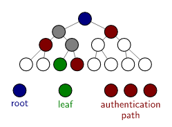
    Fast Reed-Solomon IOP of Proximity (FRI) 中，Prover发送a sequence of Merkle roots corresponding to codewords whose lengths halve in every iteration。Verifier会对相邻rounds中的Merkle tree进行检查来验证简单的线性关系（具体方法为：要求Prover提供特定叶子的authentication path）。
    对于诚实的Prover来说，其表示的多项式的degree在每一轮减半，因此远小于codeword的length。而对于malicious Prover，其degree为 codeword length - 1。最后一轮，Prover要发送a non-trivial codeword corresponding to a constant polynomial。

• Cryptographic proof system：经由 Cryptographic Compilation with FRI ，Polynomial IOP被编译为 an interactive concrete proof system。可通过Fiat-Shamir transform转换为non-interactive proof，从而命名为STARK。
  

3. STARK中的基basic tools

3.1 有限域

STARK中使用的素数域应满足$p=f\cdot 2^k+1$，其中$k$应足够大。即 存在order 为$2^k$的subgroup。

扩展域：
EthSTARK operates over the finite field defined by a 62-bit prime, but the FRI step operates over a quadratic extension field thereof in order to target a higher security level.

3.2 单变量多项式

单变量多项式可表示为：
$f(X)=c_0+c_1\cdot X+\cdots +c_d{X}^d={\sum }_{i=0}^d{c}_i{X}^i$
其中$c_i$为多项式系数，$d$为多项式degree。

STARK中，要求对domain中所有点进行evaluation，而不是对单个点进行evaluation。

Vanishing polynomial：
$Z_D(X)={\prod }_{d\in D}(X-d)$为首项系数为1的unique lowest-degree polynomial that takes the value $0$ in all points of $D$。

3.3 多变量多项式

初始状态$(a_0,b_0)$，每一轮进行如下运算：
$(a,b)\to (\frac{a+b}{2},\sqrt{a\cdot b})$

令前一轮状态为$(X_0,X_1)$经由运算后状态为$(Y_0,Y_1)$，可用多变量多项式表示为：
$m_0(X_0,X_1,Y_0,Y_1)=Y_0-\frac{X_0+X_1}{2}$
$m_1(X_0,X_1,Y_0,Y_1)=Y_1^2-X_0\cdot X_1$（注意$m_1(X_0,X_1,Y_0,Y_1)=Y_1-\sqrt{X_0\cdot X_1}$不是多项式。）

多变量多项式的表示方式可为：

class MPolynomial:
    def __init__( self, dictionary ):
        # Multivariate polynomials are represented as dictionaries with exponent vectors
        # as keys and coefficients as values. E.g.:
        # f(x,y,z) = 17 + 2xy + 42z - 19x^6*y^3*z^12 is represented as:
        # {
    
    
        #     (0,0,0) => 17,
        #     (1,1,0) => 2,
        #     (0,0,1) => 42,
        #     (6,3,12) => -19,
        # }
        self.dictionary = dictionary

3.4 Merkle tree

4. FRI

采用基于FRI的compiler可将Polynomial IOP转换为a concrete proof system。

FRI协议用于确认a committed polynomial具有bounded degree。

FRI全称为Fast Reed-Solomon IOP of Proximity，其中IOP表示interactive oracle proof。

FRI采用codewords来表示，Verifier无法读取Prover发来的所有codewords，Verifier会make oracle-queries to read them in select locations。
FRI中的codewords为Reed-Solomon codewords，即其值对应为the evaluation of some low-degree polynomial in a list of points called the domain $D$。该list的length要大于多项式中可能的非零值系数的个数 $\rho$倍，$\rho$称为expansion factor（或blowup factor）。
【即有：initial_codeword_length = (degree + 1) * expansion_factor】

codewords表示low-degree polynomials。codewords采用merkle treel来实例化。

常规的Polynomial commitment scheme为：

• polynomial commitment及实现方式对比

而FRI scheme有所不同。FRI用于证明某codeword属于a polynomial of low degree。所谓low，是指degree 值不高于 $\rho \cdot len(codeword)$。Prover知道codeword具体内容，而Verifier仅知道Merkle root和其选择的leaf。通过authentication path verification来确认the leaf’s membership to the Merkle tree。

4.1 Split-and-Fold

proof system中很赞的一个思想是：split-and-fold技术。可：（假设待证明的claim size为$n$）

• 1）将a claim reduce为 two claims of half the size。
• 2）然后利用Verifier提供的random challenge合并为一个claim。
• 3）重复以上步骤${\log }_2(n)-1$次，可最终reduce为a trivial size claim，其为true 当且仅当 原始claim为true。

对于FRI，相应的computational claim为：某特定codeword对应为a polynomial of low degree。令$N$为codeword length。$d$为该对应多项式的最大degree，表示为$f(X)={\sum }_i^d{c}_i{X}^i$。

根据FFT的divide-and-conquer策略，可将多项式分为奇数项和偶数项表示：
$f(X)=f_E(X^2)+X\cdot f_O(X^2)$
其中：
$f_E(X^2)=\frac{f(X)+f(-X)}{2}={\sum }_{i=0}^{\frac{d+1}{2}-1}{c}_{2i}{X}^{2i}$
$f_O(X^2)=\frac{f(X)-f(-X)}{2X}={\sum }_{i=0}^{\frac{d+1}{2}-1}{c}_{2i+1}{X}^{2i}$

FRI协议的关键是根据codeword for $f(X)$ 来派生 codeword for $f^{\ast }(X)=f_E(X)+\alpha \cdot f_O(X)$。其中$\alpha$为由Verifier提供的random scalar。

假设$D$为某multiplicative group的subgroup，$D$ 具有even order $N$。令$\omega$为生成subgroup $D$的generator： ⟨ ω ⟩ = D ⊂ F p \ { 0 } \langle \omega \rangle = D \subset \mathbb{F}_p \backslash\lbrace 0\rbrace ⟨ω⟩=D⊂Fp​\{ 0}。
令 { f ( ω i ) } i = 0 N − 1 \lbrace f(\omega^i)\rbrace_{i=0}^{N-1} { f(ωi)}i=0N−1​ 为$f(X)$的codeword，其实对应为evaluation on $D$。

令 $D^{\star }=⟨{\omega }^2⟩$ 为另一domain，其length为$D$的一半。
令 { f E ( ω 2 i ) } i = 0 N / 2 − 1 \lbrace f_ E(\omega^{2i})\rbrace_{i=0}^{N/2-1} { fE​(ω2i)}i=0N/2−1​， { f O ( ω 2 i ) } i = 0 N / 2 − 1 \lbrace f_ O(\omega^{2i})\rbrace_{i=0}^{N/2-1} { fO​(ω2i)}i=0N/2−1​ 和 { f ⋆ ( ω 2 i ) } i = 0 N / 2 − 1 \lbrace f^\star(\omega^{2i})\rbrace_ {i=0}^{N/2-1} { f⋆(ω2i)}i=0N/2−1​ 分别为 the codewords for $f_E(X)$，$f_O(X)$ 和 $f^{\star }(X)$，其实对应为evaluation on $D^{\star }$。

将 $f^{\star }(X)$ 的定义扩展为：
{ f ⋆ ( ω 2 i ) } i = 0 N / 2 − 1 = { f E ( ω 2 i ) + α ⋅ f O ( ω 2 i ) } i = 0 N / 2 − 1 . \lbrace f^\star(\omega^{2i})\rbrace_{i=0}^{N/2-1} = \lbrace f_E(\omega^{2i}) + \alpha \cdot f_O(\omega^{2i})\rbrace_{i=0}^{N/2-1} . { f⋆(ω2i)}i=0N/2−1​={ fE​(ω2i)+α⋅fO​(ω2i)}i=0N/2−1​.

再次根据$f_E(X^2)$ 和 $f_O(X^2)$ 的定义将 $f^{\star }(X)$ 扩展为：
{ f ⋆ ( ω 2 i ) } i = 0 N / 2 − 1 \lbrace f^\star(\omega^{2i})\rbrace_{i=0}^{N/2-1} { f⋆(ω2i)}i=0N/2−1​
$$={\left\{\frac{f({\omega }^i)+f(-{\omega }^i)}{2}+\alpha \cdot \frac{f({\omega }^i)-f(-{\omega }^i)}{2{\omega }^i}\right\}}_{i=0}^{N/2-1}$$
= { 2 − 1 ⋅ ( ( 1 + α ⋅ ω − i ) ⋅ f ( ω i ) + ( 1 − α ⋅ ω − i ) ⋅ f ( − ω i ) ) } i = 0 N / 2 − 1 = \lbrace 2^{-1} \cdot \left( ( 1 + \alpha \cdot \omega^{-i} ) \cdot f(\omega^i) + (1 - \alpha \cdot \omega^{-i} ) \cdot f(-\omega^i) \right) \rbrace_{i=0}^{N/2-1} ={ 2−1⋅((1+α⋅ω−i)⋅f(ωi)+(1−α⋅ω−i)⋅f(−ωi))}i=0N/2−1​

由于$\omega$的order为$N$，因此有${\omega }^{N/2}=-1$，从而有$f(-{\omega }^i)=f({\omega }^{N/2+i})$。因此，尽管iterate index减半为由$0$到$N/2-1$，但是所有的points并未减半，仍为 { f ( ω i ) } i = 0 N − 1 \{f(\omega^i)\}_{i=0}^{N-1} { f(ωi)}i=0N−1​。所有的这些points用于派生 { f ⋆ ( ω 2 i ) } i = 0 N / 2 − 1 \lbrace f^\star(\omega^{2i})\rbrace_{i=0}^{N/2-1} { f⋆(ω2i)}i=0N/2−1​，尽管派生后的codeword仅有一半length，尽管其polynomial仅有half the degree。

以FRI protocol中的一轮为例：

• 1）Prover commit to $f(X)$：将其codeword { f ( ω i ) } i = 0 N − 1 \lbrace f(\omega^i)\rbrace_{i=0}^{N-1} { f(ωi)}i=0N−1​ 的merkle root发送给Verifier。
• 2）Verifier发送challenge $\alpha$。
• 3）Prover计算并commit to $f^{\star }(X)$：将其codeword { f ⋆ ( ω 2 i ) } i = 0 N / 2 − 1 \lbrace f^\star(\omega^{2i})\rbrace_{i=0}^{N/2-1} { f⋆(ω2i)}i=0N/2−1​ 的merkle root发送给Verifier。
• 4）Verifier此时有2组polynomial commitments，接下来要验证两者之间的关系是否正确：
  $f^{\star }(X)=2^{-1}\cdot \left((1+\alpha X^{-1})\cdot f(X)+(1-\alpha X^{-1})\cdot f(-X)\right)$
  为此，Verifier需随机选择一个index i ← R { 0 , … , N / 2 − 1 } i \xleftarrow{R} \lbrace 0, \ldots, N/2-1\rbrace iR ​{ 0,…,N/2−1}，【注意，index的选择是与round关联的。如果index的选择与round不相关，则可能会存在fail to catch hybrid codewords的情况。实时上，可在所有轮中复用相同的index，必要时基于codeword length 进行modulo运算。】
  从而可确定3个point：
  • $A:({\omega }^i,f({\omega }^i))$
  • $B:({\omega }^{N/2+i},f({\omega }^{N/2+i}))$
  • $C:(\alpha ,f^{\star }({\omega }^{2i}))$
    注意，$A和B$的$x$坐标为${\omega }^{2i}$的平方根。
• 5）Prover收到Verifier发来的index $i$之后，仅需提供Merkle authentication paths的$y$坐标。
• 6）Verifier验证该authentication path与root匹配，同时验证$A,B,C$在同一条直线上（又称为colinearity check）。
  colinearity check成立的原因在于：穿过A、B的直线可表示为：
  $$\begin{gathered} y=\sum _i{y}_i\prod _{j\ne i}\frac{x-x_j}{x_i-x_j} \\ =f({\omega }^i)\cdot \frac{x-{\omega }^{N/2+i}}{{\omega }^i-{\omega }^{N/2+i}}+f({\omega }^{N/2+i})\cdot \frac{x-{\omega }^i}{{\omega }^{N/2+i}-{\omega }^i} \\ =f({\omega }^i)\cdot 2^{-1}\cdot {\omega }^{-i}\cdot (x+{\omega }^i)-f({\omega }^{N/2+i})\cdot 2^{-1}\cdot {\omega }^{-i}(x-{\omega }^i) \\ =2^{-1}\cdot \left((1+x\cdot {\omega }^{-i})\cdot f({\omega }^i)+(1-x\cdot {\omega }^{-i})\cdot f({\omega }^{N/2+i})\right). \end{gathered}$$
  当$x=\alpha$时，即有$y=f^{\star }({\omega }^{2i})$，从而说明$C$也在该直线上。

重复以上round即可。一共需要${\log }_2(d+1)-1$轮，其中$d$为原始多项式的degree。最终获得的为constant polynomial，其codeword也为constant。最后一轮中，Prover直接将该constant而不是merkle root发送给Verifier即可。

4.2 FRI Security Level

需要多少个colinearity checks才能达到$\lambda$ security level？目前暂无定论。

对于code rate $\rho$，ethSTARK Documentation——Version 1.1中的安全猜想为：

• The hash function used for building Merkle trees needs to have at least $2\lambda$ output bits.
• The field needs to have at least $2^{\lambda }$ elements. (Note that this refers tot the field used for FRI. In particular, you can switch to an extension field if the base field is not large enough.)
• You get ${\log }_2{\rho }^{-1}$ bits of security for every colinearity check, so setting setting the number of colinearity checks to $s=\lceil \lambda /{\log }_2{\rho }^{-1}\rceil$ achieves $\lambda$ bits of security.

因此，实际round值为：【要结合num_colinearity_tests来确认。】

	def num_rounds( self ):
        codeword_length = self.domain_length
        num_rounds = 0
        while codeword_length > self.expansion_factor and 4*self.num_colinearity_tests < codeword_length:
            codeword_length /= 2
            num_rounds += 1
        return num_rounds

4.3 Coset-FRI

以上定义的FRI protocol中，codewords为a list of values taken by a polynomial of low degree on a given evaluation domain $D$，其中$D$为order为$2^k$的subgroup，生成$D$的generator为$\omega$。

但是，当将FRI与STARK一起结合使用时，由于STARK protocol中也定义了Reed-Solomon codeword，可能会存在point evaluation 相交的问题。

因此，定义coset subgroup D = { g ⋅ ω i ∣ i ∈ Z } D = \lbrace g \cdot \omega^i \vert i \in \mathbb{Z}\rbrace D={ g⋅ωi∣i∈Z}，其中$g$为整个multiplicative group F \ { 0 } \mathbb{F} \backslash \lbrace 0\rbrace F\{ 0}的generator。而下一轮codeword所选择的evaluation domain 为the set of squares of $D$：
D ⋆ = { d 2 ∣ d ∈ D } = { g 2 ⋅ ω 2 i ∣ i ∈ Z } D^\star = \lbrace d^2 \vert d \in D\rbrace = \lbrace g^2 \cdot \omega^{2i} \vert i \in \mathbb{Z}\rbrace D⋆={ d2∣d∈D}={ g2⋅ω2i∣i∈Z}

5. STARK Polynomial IOP

采用基于FRI的compiler可将Polynomial IOP转换为a concrete proof system。

5.1 Arithmetic Intermediate Representation (AIR)

Arithmetic Intermediate Representation (AIR)，又名 arithmetic internal representation，用于：
describe a computation in terms of an execution trace that satisfies a number of constraints induced by the correct evolution of the state。

arithmetic是指：

• execution trace中包含了a list of finite field elements（如果包含了多于1个register，则为an array）。
• 可使用low degree polynomials来表示constraints。

令${\mathbb{F}}_p$为有限域，computation描述了the evolution a state of $\mathsf{w}$ registers for $T$ cycles。
algebraic execution trace (AET) 为包含$T\times \mathsf{w}$个field elements的table。其中每一行描述了the state of the system at the given point in time，每一列tracks the value of the given register。

state transition function 定义了the state at the next cycle as a function of the state at the previous cycle：
$$f:{\mathbb{F}}_p^{\mathsf{w}}\to {\mathbb{F}}_p^{\mathsf{w}}$$

同时，边界条件enforce了第一轮、最后一轮或者任意某一轮 的 某些或所有registers 的正确值：
$$\mathcal{B}:[{\mathbb{Z}}_T\times {\mathbb{Z}}_{\mathsf{w}}\times \mathbb{F}]$$

computational integrity claim中包含了：

• state transition function
• 边界条件

computational integrity claim 的witness为 algebraic execution trace。若存在a witness $W\in {\mathbb{G}}^{T\times w}$满足如下条件，则claim为true：

• for every cycle, the state evolves correctly: ∀ i ∈ { 0 , … , T − 1 }   .   f ( W [ i , : ] ) = W [ i + 1 , : ] \forall i \in \lbrace 0, \ldots, T-1 \rbrace \, . \, f(W_{[i,:]}) = W_{[i+1,:]} ∀i∈{ 0,…,T−1}.f(W[i,:]​)=W[i+1,:]​; and
• all boundary conditions are satisfied: $\forall (i,w,e)\in \mathcal{B}.W_{[i,w]}=e$.

state transition function隐藏了很多复杂度。STARK中，要求能使用与cycle 无关的low degree polynomial来描述state transition function。
$f:{\mathbb{F}}_p^{\mathsf{w}}\to {\mathbb{F}}_p^{\mathsf{w}}$ 被表示为一组多项式：$\mathbf{p}(X_0,\dots ,X_{\mathsf{w}-1},Y_0,\dots ,Y_{\mathsf{w}-1})$ such that $f(\mathbf{x})=\mathbf{y}$ if and only if $\mathbf{p}(\mathbf{x},\mathbf{y})=0$。具有$r$个state transition verification polynomials。然后，相应的transition constraints变为：

• ∀ i ∈ { 0 , … , T − 1 }   .   ∀ j ∈ { 0 , … , r − 1 }   .   p j ( W [ i , 0 ] , … , W [ i , w − 1 ] , W [ i + 1 , 0 ] , … , W [ i + 1 , w − 1 ] ) = 0 \forall i \in \lbrace 0, \ldots, T - 1 \rbrace \, . \, \forall j \in \lbrace 0, \ldots, r-1\rbrace \, . \, p_j(W_{[i,0]}, \ldots, W_{[i, \mathsf{w}-1]}, W_{[i+1,0]}, \ldots, W_{[i+1, \mathsf{w}-1]}) = 0 ∀i∈{ 0,…,T−1}.∀j∈{ 0,…,r−1}.pj​(W[i,0]​,…,W[i,w−1]​,W[i+1,0]​,…,W[i+1,w−1]​)=0.

这种表达方式是非确定性的，即存在空间来将 high degree state transition computation polynomial reduce为 low degree state transition verification polynomial。
如，对于state transition function $f:{\mathbb{F}}_p\to {\mathbb{F}}_p$：
$$x\mapsto \{\begin{array}{lc}{x}^{-1}& \Leftarrow x\ne 0\\ 0& \Leftarrow x=0\end{array}$$
可采用computation polynomial 表示：$f(x)=x^{p-1}$
或采用verification polynomial 表示：$\mathbf{p}(x,y)=(x(xy-1),y(xy-1))$
从而将degree 由 $p-1$ 降为 $3$。

5.2 Interpolation

arithmetic constraint system 将 computational integrity claim 表示为 a bunch of polynomials，每个polynomial 对应一个constraint。
将constraint system转换为Polynomial IOP需要将polynomial extend为witness，将valid witness extend为witness polynomial。
需要将 the conditions for true computational integrity claims表示为polynomial identities。

令$D$为trace evaluation domain。$D$的generator为$o$，其order为$2^k\ge T+1$。
令 D = { ο i ∣ i ∈ Z } D = \lbrace \omicron^i \vert i \in \mathbb{Z}\rbrace D={ οi∣i∈Z}。The Greek letter $o$ (“omicron”) indicates that the trace evaluation domain is smaller than the FRI evaluation domain by a factor exactly equal to the expansion factor（$\rho$）。

令$\mathbf{t}(X)\in ({\mathbb{F}}_p[X]{)}^{\mathsf{w}}$ 为$\mathsf{w}$个单变量多项式，interpolate through $W$ on $D$。对register $w$的trace polynomial $t_w(X)$为lowest degree 单变量多项式，使得 ∀ i ∈ { 0 , … , T }   .   t w ( ο i ) = W [ i , w ] \forall i \in \lbrace 0, \ldots, T\rbrace \, . \, t_w(\omicron^i) = W[i, w] ∀i∈{ 0,…,T}.tw​(οi)=W[i,w]。trace polynomial 可将algebraic execution trace表示为单变量多项式。

将the conditions for true computational integrity claims 转换为 trace polynomials，满足：

• all boundary constraints are satisfied: $\forall (i,w,e)\in \mathcal{B}.t_w(o^i)=e$; and
• for all cycles, all transition constraints are satisfied: ∀ i ∈ { 0 , … , T − 1 }   .   ∀ j ∈ { 0 , … , r − 1 }   .   p j ( t 0 ( ο i ) , … , t w − 1 ( ο i ) , t 0 ( ο i + 1 ) , … , t w − 1 ( ο i + 1 ) ) = 0 \forall i \in \lbrace 0, \ldots, T-1 \rbrace \, . \, \forall j \in \lbrace 0, \ldots, r-1 \rbrace \, . \, p_j( t_0(\omicron^i), \ldots, t_{\mathsf{w}-1}(\omicron^i), t_0(\omicron^{i+1}), \ldots, t_{\mathsf{w}-1}(\omicron^{i+1})) = 0 ∀i∈{ 0,…,T−1}.∀j∈{ 0,…,r−1}.pj​(t0​(οi),…,tw−1​(οi),t0​(οi+1),…,tw−1​(οi+1))=0.【等式左侧的部分可看成是单变量多项式$p_j(t_0(X)),\dots ,t_{\mathsf{w}-1}(X),t_0(o\cdot X),\dots ,t_{\mathsf{w}-1}(o\cdot X))$。整个表达式 表示 所有$r$个 transition polynomials evaluate to 0 in { ο i ∣ i ∈ Z T } \lbrace \omicron^i \vert i \in \mathbb{Z}_T\rbrace { οi∣i∈ZT​}。】

基于以上观察，有high-level Polynomial IOP：

• 1）The prover commits to the trace polynomials $\mathbf{t}(X)$.
• 2）The verifier checks that $t_w(X)$ evaluates to $e$ in $o^i$ for all $(i,w,e)\in \mathcal{B}$.
• 3）The prover commits to the transition polynomials $\mathbf{c}(X)=\mathbf{p}(t_0(X)),\dots ,t_{\mathsf{w}-1}(X),t_0(o\cdot X),\dots ,t_{\mathsf{w}-1}(o\cdot X))$.【实际上，对transition polynomials的commitment可湖绿，Verifier可使用$\mathbf{t}(X)$在$z$和$o\cdot z$的evaluation值来计算 $\mathbf{c}(X)$在某点的值，从而可验证 $\mathbf{c}(X)$ evaluate to 0 in { ο i ∣ i ∈ { 0 , … , T − 1 } } \lbrace \omicron^i \vert i \in \lbrace 0, \ldots, T-1 \rbrace \rbrace { οi∣i∈{ 0,…,T−1}}。】
• 4）The verifier checks that $\mathbf{c}(X)$ and $\mathbf{t}(X)$ are correctly related by:
  • choosing a random point $z$ drawn uniformly from the field excluding the element 0,
  • querying the values of $\mathbf{t}(X)$ in $z$ and $o\cdot z$,
  • evaluating the transition verification polynomials $\mathbf{p}(X_1,\dots ,X_{\mathsf{w}-1},Y_0,\dots ,Y_{\mathsf{w}-1})$ in these $2\mathsf{w}$ points, and
  • querying the values of $\mathbf{c}(X)$ in $z$,
  • checking that the values obtained in the previous two steps match;
• 5）The verifier checks that the transition polynomials $\mathbf{c}(X)$ evaluate to zero in { ο i ∣ i ∈ { 0 , … , T − 1 } } \lbrace \omicron^i \vert i \in \lbrace 0, \ldots, T-1 \rbrace \rbrace { οi∣i∈{ 0,…,T−1}}.

FRI compiler 可按如下步骤 模拟 an evaluation check：

• a）减去$y$坐标。
• b）除以 zerofier。所谓zerofier，为the minimal polynomial that vanishes at the $x$-coordinate。
• c）证明步骤b）中得到的quotient polynomial 具有a bounded degree。

在STARK中，以上evaluation check流程需要发生2次：

• 1）用于trace polynomials，来表示satisfaction of the boundary constraints。获得的quotient polynomials称为boundary quotients。
• 2）用于transition polynomials，用于表示transition constraints are satisfied。获得的quotient polynomials称为transition quotients。

二者之间有冗余，trace polynomials与2组quotient polynomials均相关。因此可二者进行合并，删除冗余重复的部分，实际STARK Polynomial IOP的工作流为：【绿色盒子中的boundary quotients 和 transition quotients会进行evaluation并将其Merkle root作为其commitment值。该Merkle root是FRI的输入。
上部的红色字体内容与arithmetic constraint system关联。】

Verifier仅需验证the boundary quotients and the transition quotients are linked。由boundary quotients，通过运行特定的运算，可生成transition quotients，从而构建了二者之间的link关系。

整个工作流中会生成2个recipes，一个给 Prover，一个给Verifier。

Prover端：

• Interpolate the execution trace to obtain the trace polynomials.
• Interpolate the boundary points to obtain the boundary interpolants, and compute the boundary zerofiers along the way.
• Subtract the boundary interpolants from the trace polynomials, giving rise to the dense trace polynomials.
• Divide out the boundary zerofiers from the dense trace polynomials.
• Commit to the dense trace polynomials.
• Get $r$ random coefficients from the verifier.
• Compress the $r$ transition constraints into one master constraint that is the weighted sum.
• Symbolically evaluate the master constraint in the trace polynomials, thus generating the transition polynomial.
• Divide out the transition zerofier to get the transition quotient.
• Commit to the transition zerofier.
• Run FRI on all committed polynomials.
• Supply the Merkle leafs and authentication paths that are requested by the verifier.

Verifier端：

• Read the commitments to the boundary quotients.
• Supply the random coefficients for the master transition constraint.
• Read the commitment to the transition quotient.
• Run the FRI verifier.
• Verify the link between boundary quotients and transition quotient. To do this:
  • For all points of the transition quotient codeword that were queried in the first round of FRI do:
    • Let the point be $(x,y)$.
    • Query the matching points on the boundary quotient codewords. Note that there are two of them, $x$ and $o\cdot x$, indicating points “one cycle apart”.
    • Multiply the y-coordinates of these points by the zerofiers’ values in $x$ and $o\cdot x$.
    • Add the boundary interpolants’ values.
    • Evaluate the master transition constraint in this point.
    • Divide by the value of the transition zerofier in $x$.
    • Verify that the resulting value equals $y$.

5.3 Generalized AIR Constraints

AIR Constraints中包含了2个多项式：

• 分子多项式：确定了which equations between elements of the algebraic execution trace hold, in a manner that is independent of the cycle。对于transition constraints，分子为exactly the transition constraint polynomial；对于boundary constraints，分子为$t_i(X)-y$，其中$y$为the value of $t_i(X)$ at the given boundary。
• 分母多项式：a zerofier that determines where the equality is supposed to hold, by vanishing (i.e., evaluating to zero) in those points. 对于transition constraints，该zerofier vanishes on all points of the trace evaluation domain except the last；对于boundary constraints, this zerofier vanishes only on the boundary。

可将boundary constraints和transition constraints作为generalized AIR constraints的一个子类，从而可形成更简单的工作流：

此时，Prover commits to the raw trace polynomials, but these polynomials are not input to the FRI subprotocol. Instead, they are used to only verify that the leafs of the first Merkle tree of FRI were computed correctly.

5.4 STARK + Zero Knowledge

所谓Zero Knowledge，是指Prover引入randomizer，可在不泄露witness的前提下证明proof的正确性。

对于STARK proof system，可在如下2个维度引入randomizer：

• 1）FRI bounded degree proof：为nonlinear combination中增加a randomizer codeword。该randomizer codeword对应a polynomial of maximal degree whose coefficients are drawn uniformly at random。
• 2）构建boundary quotients到transition quotient(s)的linking part：每个register的execution需扩展$4s$个uniformly random field elements。$4s$源于：FRI protocol中有$s$个colinearity checks，每个colinearity check在初始codeword中会引发2次query。这2次query产生的2个transition quotient codeword值需要关联4个boundary quotient codeword值。

It is important to guarantee that none of the x-coordinates that are queried as part of FRI correspond to x-coordinates used for interpolating the execution trace. This is one of the reasons why coset-FRI comes in handy. Nevertheless, other solutions can address this problem.

Lastly, if the field is not large enough (specifically, if its cardinality is significantly less than $2^{\lambda }$ for security level $\lambda$), then salts need to be appended to the leafs when building the Merkle tree. Specifically, every leaf needs $\lambda$ bits of randomness, and if it does not come from the field element then it must come from an explicit appendix.

Without leaf salts, the Merkle tree and its paths are deterministic for a given codeword. This codeword is still somewhat random, because the polynomial that generates it has randomizers. However, every leaf has at most $|{\mathbb{F}}_p|$ bits of entropy, and when this number of smaller than $\lambda$, the attacker is likely to find duplicate hash digests. In other words, he can notice, with less than $2^{\lambda }$ work, that the same value is being input to the hash function. This observation leads to a distinguisher between authentic and simulated transcript, which in turn undermines zero-knowledge.

参考资料

[1] Anatomy of a STARK
[2] Awesome StarkNet