Python之matplotlib模块介绍及简单应用
在这里,我们将要介绍五个简单的案例及其实现
(五个绘图实例,二个二维,三个三维)
一、还是老规矩,首先安装matplotlib库
安装matplotlib库
控制器命令:pip install matplotlib
要是Linux的,我还真不会~~
示例图如下:

二、matplotlib模块简介
Matplotlib 是 Python 的绘图库。 它可与 NumPy 一起使用,提供了一种有效的 MatLab 开源替代方案。 它也可以和图形工具包一起使用,如 PyQt 和 wxPython。
总之就是说,它是一个绘图的库,可以用来绘图,这里我们采用与numpy合用的方式来绘图。
至于numpy模块的使用,可以参见我的另一篇博文:
“python 之 numpy 模块详细讲解及其应用案例”
链接为:https://blog.csdn.net/m0_54218263/article/details/114272263
里面有详细讲解,同时也少量的应用了一点点matplotlib模块
三、matplotlib模块的实例
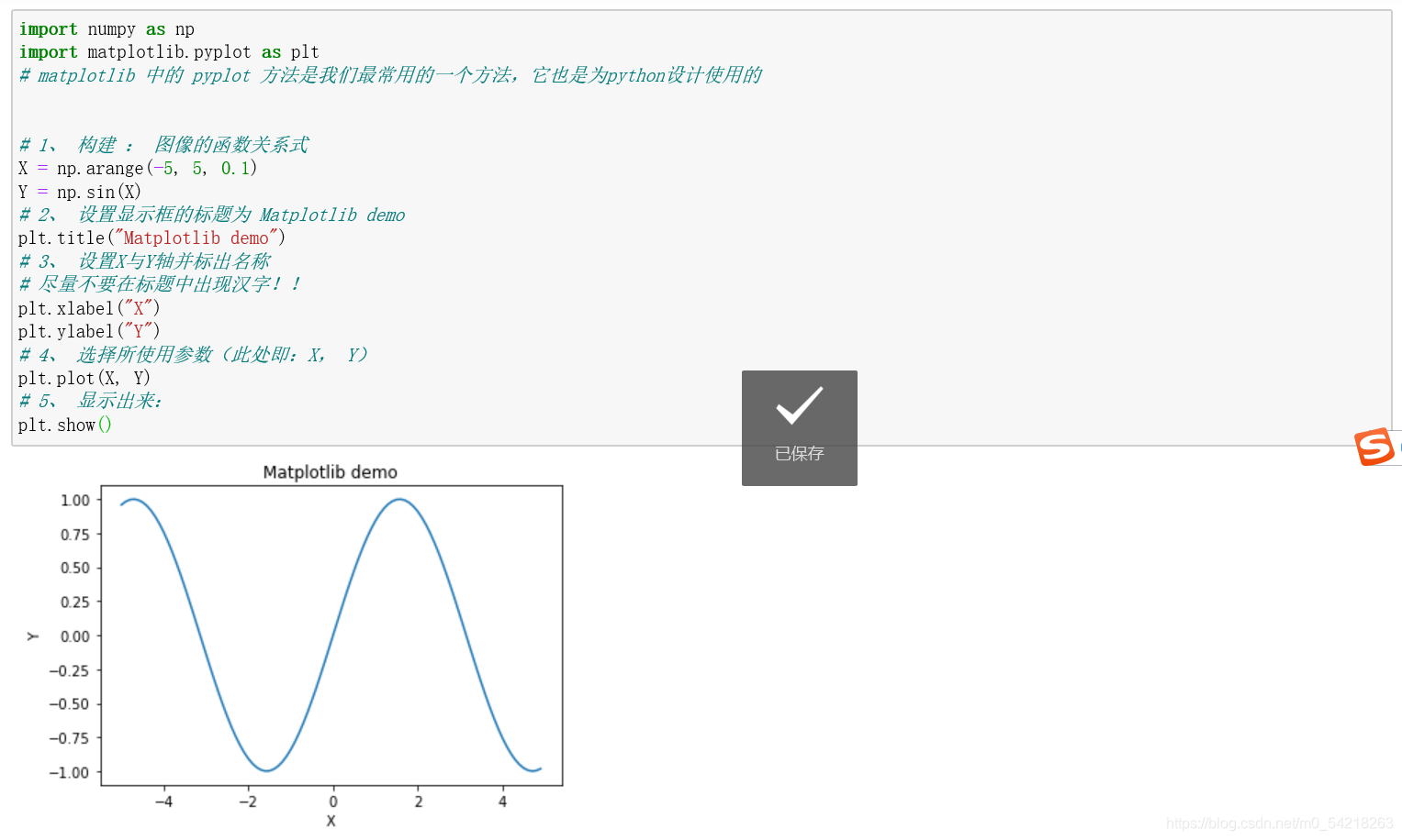
第一个实例:
二维连续图像
(显示一个二维的图像,连续的)
"""
导入模块
这里采用的模块的别名
是业界常用的操作
"""

import numpy as np
import matplotlib.pyplot as plt
# matplotlib 中的 pyplot 方法是我们最常用的一个方法,它也是为python设计使用的


# 1、 构建 : 图像的函数关系式
X = np.arange(-5, 5, 0.1)
Y = np.sin(X)

# 2、 设置显示框的标题为 Matplotlib demo
plt.title("Matplotlib demo")

# 3、 设置X与Y轴并标出名称
# 在这里尽量不要在标题中出现汉字!!否则会有乱码出现!!
plt.xlabel("X")
plt.ylabel("Y")

# 4、 选择所使用参数(此处即:X, Y)
plt.plot(X, Y)

# 5、 显示出来:
plt.show()
结果展示如下所示:

在上例中,如果将语句:X = np.arange(-5, 5, 0.1) 改为:
X = np.arange(-5, 5, 1),则图像会有很大改变,如下所示(偏离了我们的期望):

所以说,合理的取点也很重要!!
第二个实例:
二维离散图像
(显示一个二维的图像,离散的)
本案例与前一个案例较为相似,故不多做解释了~~
import numpy as np
import matplotlib.pyplot as plt

# 为了可以看清楚,这里将间隔改为了 0.5
# 即:第三个参数变为 0.5
X = np.arange(-5, 5, 0.5)
Y = np.sin(X)

# 标题和坐标轴信息:
plt.title("Demo 2")
plt.xlabel("X")
plt.ylabel("Y")


# 参数'ob'表示使用散点图的形式输出图形!!

"""
一般默认为曲线
但有参数则为不同样式(例如:‘ob’)
o--->用圆点表示
b--->颜色是蓝色的
其他的字符表示方法请参见本案例的结尾处附表!!
"""

plt.plot(X, Y, 'ob')

plt.show()
运行结果如下所示:


附表(字符表示的含义,这个是从别的地方截图过来的)


第三个实例:
三维连续图像
(显示一个三维的图像,连续的)
首先,用前面的方法会报错:

(原因里面也写了,没有zlabel)
因此换用下方的方法来进行绘制:
import numpy as np
import matplotlib.pyplot as plt
# 导入库


# 建立坐标系
fig = plt.figure()
# 构建三维空间
ax_0 = plt.axes(projection='3d')
# 设置X,Y(用arange的方法来实现)
# 建议X与Y设置相同的范围和间隔!!
X = np.arange(-3, 3, 0.1)
Y = np.arange(-3, 3, 0.1)
# meshgrid方法,
"""
meshgrid方法:

相当于是在这里进行建立了一个二维的网格,(二维坐标系):
以(X, Y)为坐标单元建立的
例如:(-3, 2.9)  (-2, -1) 等等
这只是一个简单的理解

具体的讲解请参见下方的链接!!!
参见下方链接!!!
"""
x,y = np.meshgrid(X, Y)
# 写出z的函数表达式
z = np.exp(100 - x ** 2 - y ** 2)
# 绘制图像,cmap参数是设置图形的样式的,rainbow为彩虹状
ax_0.plot_surface(x, y, z, cmap='rainbow')
# 展示出来图像
plt.show()
"""
cmap取值
这里展示的十分全面,可以从中挑选作为cmap的值
cmap 的可取值如下:

'Accent', 'Accent_r', 'Blues', 'Blues_r', 'BrBG',
'BrBG_r', 'BuGn', 'BuGn_r', 'BuPu', 'BuPu_r', 'CMRmap',
'CMRmap_r', 'Dark2', 'Dark2_r', 'GnBu', 'GnBu_r', 'Greens',
'Greens_r', 'Greys', 'Greys_r', 'OrRd', 'OrRd_r', 'Oranges',
'Oranges_r', 'PRGn', 'PRGn_r', 'Paired', 'Paired_r', 'Pastel1',
'Pastel1_r', 'Pastel2', 'Pastel2_r', 'PiYG', 'PiYG_r', 'PuBu',
'PuBuGn', 'PuBuGn_r', 'PuBu_r', 'PuOr', 'PuOr_r', 'PuRd', 'PuRd_r',
'Purples', 'Purples_r', 'RdBu', 'RdBu_r', 'RdGy', 'RdGy_r', 'RdPu',
'RdPu_r', 'RdYlBu', 'RdYlBu_r', 'RdYlGn', 'RdYlGn_r', 'Reds',
'Reds_r', 'Set1', 'Set1_r', 'Set2', 'Set2_r', 'Set3', 'Set3_r',
'Spectral', 'Spectral_r', 'Wistia', 'Wistia_r', 'YlGn', 'YlGnBu',
'YlGnBu_r', 'YlGn_r', 'YlOrBr', 'YlOrBr_r', 'YlOrRd', 'YlOrRd_r',
'afmhot', 'afmhot_r', 'autumn', 'autumn_r', 'binary', 'binary_r',
'bone', 'bone_r', 'brg', 'brg_r', 'bwr', 'bwr_r', 'cividis',
'cividis_r', 'cool', 'cool_r', 'coolwarm', 'coolwarm_r', 'copper',
'copper_r', 'cubehelix', 'cubehelix_r', 'flag', 'flag_r',
'gist_earth', 'gist_earth_r', 'gist_gray', 'gist_gray_r', 'gist_heat',
'gist_heat_r', 'gist_ncar', 'gist_ncar_r', 'gist_rainbow',
'gist_rainbow_r', 'gist_stern', 'gist_stern_r', 'gist_yarg',
'gist_yarg_r', 'gnuplot', 'gnuplot2', 'gnuplot2_r', 'gnuplot_r',
'gray', 'gray_r', 'hot', 'hot_r', 'hsv', 'hsv_r', 'inferno',
'inferno_r', 'jet', 'jet_r', 'magma', 'magma_r', 'nipy_spectral',
'nipy_spectral_r', 'ocean', 'ocean_r', 'pink', 'pink_r', 'plasma',
'plasma_r', 'prism', 'prism_r', 'rainbow', 'rainbow_r', 'seismic',
'seismic_r', 'spring', 'spring_r', 'summer', 'summer_r', 'tab10',
'tab10_r', 'tab20', 'tab20_r', 'tab20b', 'tab20b_r', 'tab20c',
'tab20c_r', 'terrain', 'terrain_r', 'turbo', 'turbo_r', 'twilight',
'twilight_r', 'twilight_shifted', 'twilight_shifted_r', 'viridis',
'viridis_r', 'winter', 'winter_r'
"""
(这两个 meshgrid 链接其实是一样的,
如果没有办法打开,可以直接输入网址进行访问)
加载的时候需要等上十几秒钟的时间!!
https://ww2.mathworks.cn/help/matlab/ref/meshgrid.html
运行后的结果如下图所示:
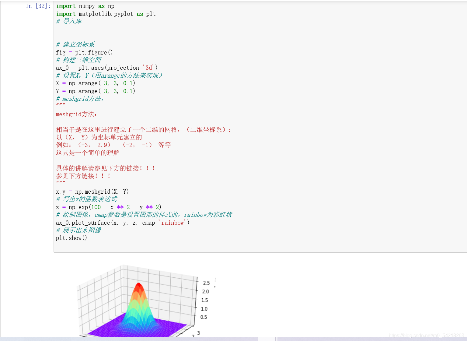

(是不是有一点点彩虹rainbow的意味在内啊~~)
第四个实例
三维离散图像
(显示一个三维的图像,离散的)
import numpy as np
import matplotlib.pyplot as plt

# plt
fig = plt.figure()
ax_1 = plt.axes(projection='3d')


"""
random方法用来产生随机数,这里意为:

产生100个从0到1的随机数
"""
zd = 13*np.random.random(100)
# 100 个0~1的随机数, 产生以后乘以13


# xd,yd的函数关系(zd是自变量)
xd = 5*np.sin(zd)
yd = 5*np.cos(zd)


ax_1.scatter3D(xd, yd, zd, cmap='Blues')  # 绘制散点图(三维的)
plt.show() # 展示图像
结果的输出如下所示:
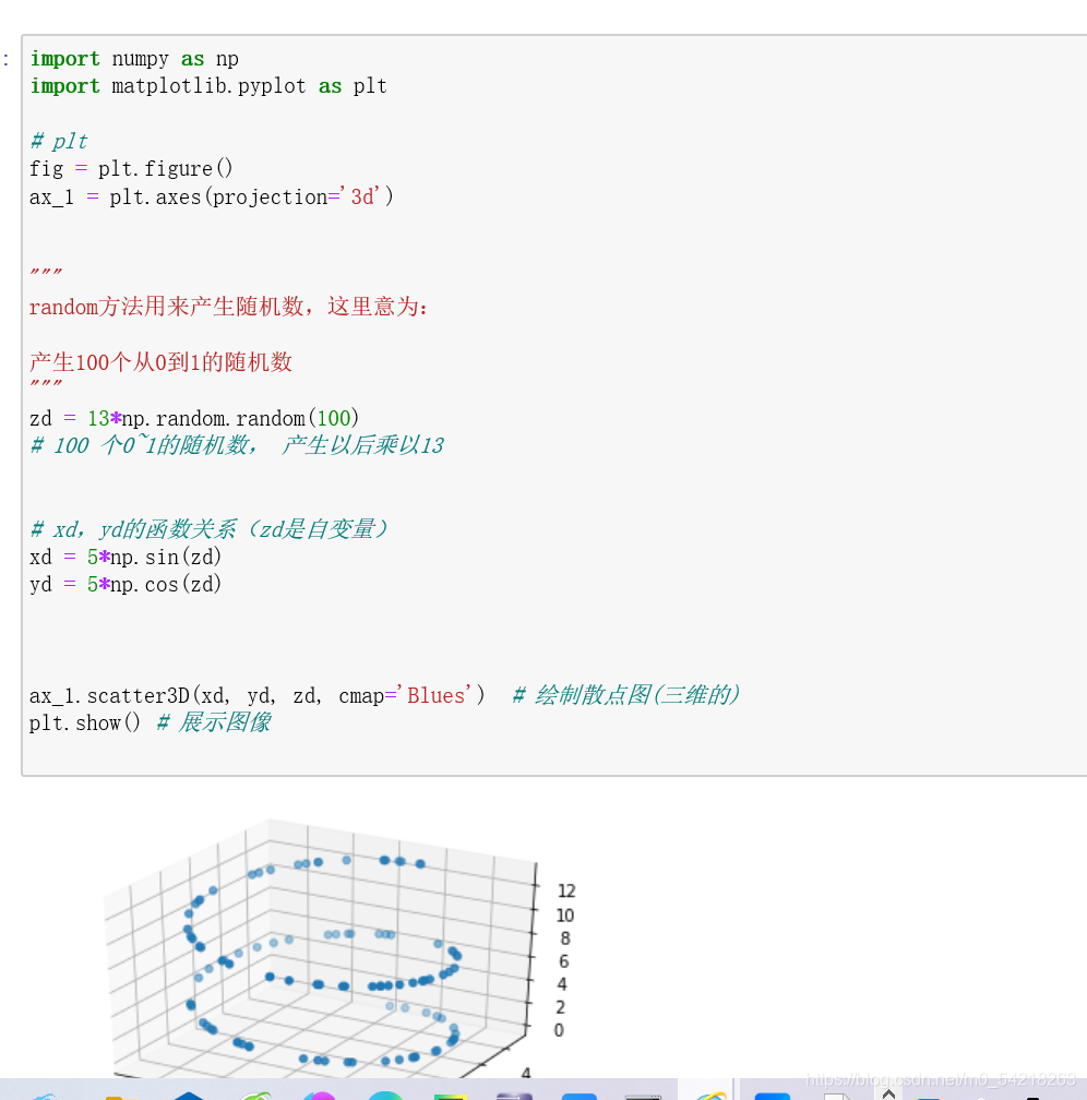
图1

图2

比较图1 以及 图2 ,我们可以发现两张图不一样,即:两张图的点的分布是不同的。
这也正是因为:random是随机产生点的;
也恰恰验证了random确实是随机的生成数字!!
第五个实例
等高线的绘制
(三维空间中,一个函数会存在各个方向上的投影,我们在这里绘制等高线图,即就是:在x,y,z三个方向的投影)
import numpy as np
import matplotlib.pyplot as plt
fig = plt.figure()
ax_2 = plt.axes(projection='3d')

# 类似于上面的代码,构建三维函数(这里购进一个三维曲面)
x = np.arange(-5, 5, 0.1)
y = np.arange(-5, 5, 0.1)
X, Y = np.meshgrid(x, y)
Z = np.log(X ** 2 + Y ** 2 + 10)

# 绘制曲面图像以及投影图:
ax_2.plot_surface(X, Y, Z, cmap='winter')     # 三维的曲面图像
ax_2.contour(X, Y, Z, zdir='z', offset=-3, cmap="rainbow")  # z方向投影,投到x-y平面
ax_2.contour(X, Y, Z, zdir='x', offset=-6, cmap="rainbow")  # x方向投影,投到y-z平面
ax_2.contour(X, Y, Z, zdir='y', offset=6, cmap="rainbow")   # y方向投影,投到x-z平面
"""
解释一下在这里的offset参数:

offset--->将投影放置在什么位置

例如:
ax_2.contour(X, Y, Z, zdir='z', offset=-3, cmap="rainbow")

意为:
将 z 方向投影(即x-y平面)的曲线的投影放置在 z = -3 的平面之上!!
"""

# 这里说明一下坐标轴的命名方法:
ax_2.set_xlabel("X")
ax_2.set_ylabel("Y")
ax_2.set_zlabel("Z")

# 展示图像:
plt.show()
运行结果展示如下所示:

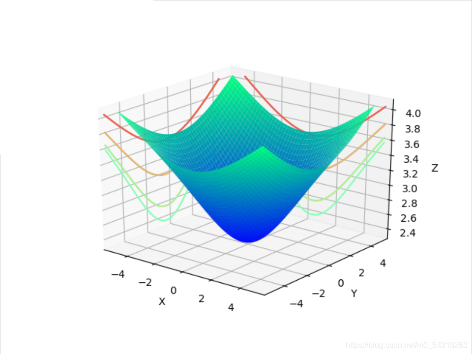


(图形可以旋转)
*综上所述,上面便是所列举的五个例子,希望对大家有所帮助~~~~*
*最后再感谢您能耐心读到最后~~~~*