深度学习大致步骤

1. 准备数据

2. 搭建模型

3. 迭代训练模型

模型是如何训练出来的

模型里的内容和意义

模型结构：输入-中间节点-输出

TensorFlow 将中间节点及节点间的运算关系(OPS)定义在自己内部的一个“图”上，全通过一个“会话(session)”行图中OPS具体运算。

可以这样理解：

"图"是静态的，无论做任何加减乘除，他们只是将关系搭建在一起，不会有任何运算
"会话"是动态的，只有启动会话后才会将数据流向图中，并按照图中的关系运算，并将最终的结果从图中流出
任何一个结点可以通过会话的run函数进行计算，得到该节点的真实数值

tensorflow的这种方式分离了定义和执行。

模型内部的数据流向

1. 正向

正向，是数据从输入开始，依次进行各节点定义的运算，一直运算到输出，是模型基本数据流向。

2. 反向

反向，只有在训练场景中才会使用到。
先从正向的最后一个节点开始，计算此时结果值与真实值的误差，这样会形成一个用计算学习参数表示误差的方程，然后对方程中的每个参数求导，得到其梯度修正值，同时反推出上一层的误差，类推直到传到正向的第一个节点。

重点

使用什么方法来计算误差
使用哪些梯度下降的优化方法
如何调节梯度下降中的参数（如学习率）

4. 使用模型

import tensorflow as tf
import numpy as np
import matplotlib.pyplot as plt

# 1.准备数据
train_X = np.linspace(-1, 1, 100) # -1到1的100个等距离数据（等差数列）
train_Y = 2 * train_X + np.random.randn(100) * 0.3  # 加入了噪声的 y = 2x

# 为数据图形化做准备
plotdata = {
    
    "batchsize":[], "loss":[]}
def moving_average(a, w = 10):
    if len(a) < w:
        return a[:]
    return [val if idx < w else sum(a[(idx - w):idx])/w for idx, val in enumerate(a)]

# 显示模拟数据点
plt.plot(train_X, train_Y, 'b.')
plt.legend()
plt.title("data")
plt.show()

# 2.搭建模型

# 占位符
X = tf.placeholder ("float") 
Y = tf.placeholder ("float") 

# 模型参数
W = tf.Variable(tf.random_normal([1]), name = "weight") 
b = tf.Variable(tf.zeros([1]) , name = "bias") 

# 前向结构
z = tf.multiply (X , W) + b

# 反向优化
cost = tf.reduce_mean(tf.square(Y-z))
learning_rate = 0.01
optimizer = tf.train. GradientDescentOptimizer(learning_rate).minimize(cost)


# 3.迭代训练模型

# 初始化所有变量
init = tf.global_variables_initializer()

# 定义参数
training_epochs = 20
display_step = 2

# 启动session
with tf.Session() as sess:
    sess.run(init)
    plotdata = {
    
    "batchsize":[], "loss":[]}
    # 向模型输入数据
    for epoch in range(training_epochs):
        for(x, y) in zip(train_X, train_Y):
            sess.run(optimizer, feed_dict = {
    
    X:x, Y:y})
            
        # 显示训练中的详细信息
        if epoch % display_step == 0:
            loss = sess.run(cost, feed_dict = {
    
    X:train_X, Y:train_Y})
            print ("Epoch:", epoch+1, "cost:", loss, "W=", sess.run(W), "b=", sess.run(b))
            if not (loss == "NA"):
                plotdata["batchsize"].append(epoch)
                plotdata["loss"].append(loss)
                
    # 图形显示
    fig = plt.figure(num = 1, figsize = (10, 6), dpi = 80)
    plt.plot(train_X, train_Y, 'b.', label = 'Original data')
    plt.plot(train_X, sess.run(W) * train_X + sess.run(b), 'r-', label = 'Fittedline')
    plt.legend()
    plt.show()

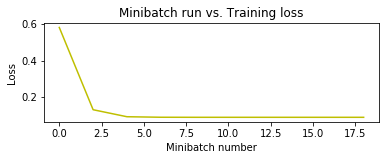
    plotdata["avgloss"] = moving_average(plotdata["loss"])
    plt.figure(1)
    plt.subplot(2, 1, 1)
    plt.plot(plotdata["batchsize"], plotdata["avgloss"], 'y-')
    plt.xlabel('Minibatch number')
    plt.ylabel('Loss')
    plt.title('Minibatch run vs. Training loss')
    plt.show()
    
    # 4.使用模型
    print ("根据已有数据推算出 输入值0.2 对应的 z值")
    print ("x = 0.2, z = ", sess.run(z, feed_dict = {
    
    X : 0.2}))

在这里插入图片描述

Epoch: 1 cost: 0.5817702 W= [0.9302488] b= [0.35420635]
Epoch: 3 cost: 0.12975623 W= [1.7124442] b= [0.14990632]
Epoch: 5 cost: 0.09125683 W= [1.9251237] b= [0.06990477]
Epoch: 7 cost: 0.088380344 W= [1.9802916] b= [0.04876148]
Epoch: 9 cost: 0.08811882 W= [1.9945589] b= [0.04328698]
Epoch: 11 cost: 0.088083476 W= [1.9982475] b= [0.04187138]
Epoch: 13 cost: 0.08807649 W= [1.9992021] b= [0.04150523]
Epoch: 15 cost: 0.088074826 W= [1.999449] b= [0.0414104]
Epoch: 17 cost: 0.08807441 W= [1.9995124] b= [0.04138604]
Epoch: 19 cost: 0.08807431 W= [1.9995282] b= [0.04137998]

在这里插入图片描述

根据已有数据推算出输入值0.2 对应的 z值
x = 0.2, z = [0.44128513]

tensorflow y = 2x大致拟合