这个领域的算法库一般有librosa、essentia、torchaudio、深度学习等。这个领域目前的工程套路是:
- 首先声音是一维的时域信号,但是计算机看了觉得没啥用(你看wav文件那些采样点,这些数字能说明啥呀);P.S. 人的听觉系统(从耳朵到大脑皮层)与之相比是多么强大呀!
- 既然一维的时域信号没啥用,于是人们开始做频域分析,也就是大名鼎鼎的fft;终于有了一些用处了,但是还是差的太远;
- 把频域和时域都加上,比如stft,最经典的时频域分析方法,怎么样?嗯,又厉害了些;
- 把时频域的分析结果转化成热力图,送给以图像分析见长的CNN网络怎么样?哇,CNN相当于人类听觉系统中的大脑皮层了,又厉害了好多;
- 但是和各种声音分析的任务比起来,还是差的比较多;那怎么弥补呢?两个方面,一是更高效的提取出声音的有效特征;二是深度学习算法的发展。在声音人工提取特征方面,几十年来进展不多,我们自然而然就放弃了;剩下的就只能仰仗深度学习算法了。
声音文件的加载
一般的声音文件要么是单声道的,要么是立体声(双声道),当然也有5.1声道的(甚至更多声道的)——只是互联网领域不多,因为手机、电脑、耳机等设备目前主要是支持立体声。
当声音文件被从wav、mp3这些容器中demux出,并且再读成pcm_s16le格式的数据时,单声道这个概念就转化为了一维数组,立体声这个概念就转化为了二维数组。当声音的采样率为44100时,那么一秒钟的立体声音频文件一般会读成一个44100x2或者2x44100的数组。
这里Gemfield使用torchaudio来举例下,使用torchaudio来读取卡农钢琴曲的mp3文件:
>>> import torch
>>> import torchaudio
>>> import matplotlib.pyplot as plt

>>> waveform, sample_rate = torchaudio.load("kalong.mp3")
>>> waveform
tensor([[0., 0., 0.,  ..., 0., 0., 0.],
        [0., 0., 0.,  ..., 0., 0., 0.]])
>>> waveform.shape
torch.Size([2, 9895643])
那么这个mp3文件的时长大概就是9895643 / sample_rate = 224秒:
>>> waveform.shape
torch.Size([2, 9895643])
>>> 9895643 / sample_rate
224.3909977324263
为了后续时频分析的方便,这些audio库大都提供的重采样的函数接口。比如resample函数就在torchaudio的transforms模块中:
torchaudio.transforms.Resample(sample_rate, new_sample_rate)(waveform)声音的特征
从幼年时期,我们学到的有关声音的知识就是声音可以看做是波,它的特征有:音频、响度、音色。
- 音频,也叫音高,波的频率,比如人耳听觉的频率范围、比如音乐的哆唻咪发嗖拉嘻等;
- 响度,波的振幅,声音的大小;
- 音色,......,解释不清,反正区分一种声音和另一种声音主要是靠音色。比如笛子和钢琴都发出相同的哆唻咪发嗖拉嘻时,我们能明显区分出这是两种不同的声音;两个歌手唱同一个音高时,我们也能却分出这是不同的声音;
只不过,上面的知识显得很苍白,因为区分声音与声音的主要标志就在上面说不清的音色里。音色是什么?没人能全部说的清楚,比如是谐波的组成比例?是包络线的形状?
一般说来,对于声音分类任务来说,主要的特征就藏在说不清楚的音色中。那怎么做呢?Gemfield从头说来。
1,声音的波形
这是最简单也是最直截了当的方式,就是挨个把采样点的值绘制在二维平面上,自然而然的就展示出了声音的波形。比如绘制出上述torchaudio读的卡农前17秒的波形图:
>>> plt.plot(waveform[:,0:44100*17].t().numpy())
[<matplotlib.lines.Line2D object at 0x1321a05d0>, <matplotlib.lines.Line2D object at 0x1321a0890>]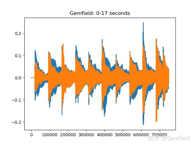
还比如,使用essentia库直截了当的绘制出卡侬钢琴曲第二个声道的第2秒的波形图:
>>> loader = essentia.standard.MonoLoader(filename='./kalong.mp3')
>>> audio = loader()
>>> from pylab import plot, show, figure, imshow
>>> import matplotlib.pyplot as plt
>>> plt.rcParams['figure.figsize'] = (15, 6)
>>> plot(audio2[0].transpose(1,0)[1][1*44100:2*44100])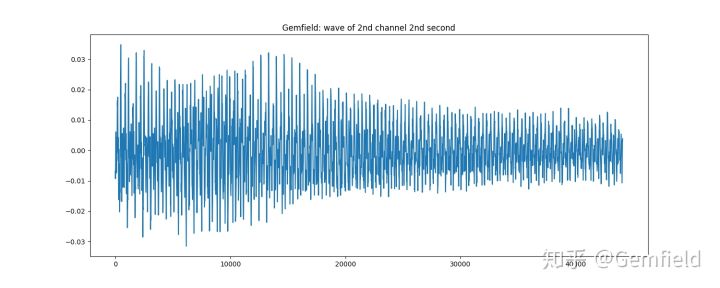
画声音波形图只是把一维的时域信号直接转化成了人喜闻乐见的形式,但是没卵用。
2,声谱图(spectrogram)
声音转换为声谱图,也是研究声音特征的一种方法。简单来说,就是将声音通过短时傅立叶变换,获得一张包含3个维度数据的热力图。如下所示:
>>> specgram = torchaudio.transforms.Spectrogram(n_fft=1024)(waveform)
>>> plt.imshow(specgram.log2()[0,:,:1000].numpy(), cmap='plasma')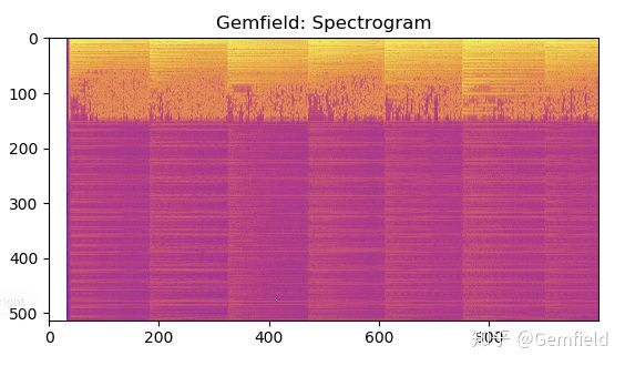
图中横轴代表时间,纵轴代表频率,颜色代表能量。
在将声音数据通过STFT(短时傅立叶变换)转换为声谱图的过程中,每个算法库都提供了类似的接口和参数,这是由stft算法的本质决定的。这些参数有:
- n_fft,frame length,也就是一帧的采样点数量;
- win_length,窗函数相关,一般和frame length等长;
- hop_length,往前跳跃的步长,一般是frame length的一半;
- window_fn,窗函数,默认是torch.hann_window(汉宁窗)。
热力图使用的调色板一般有如下这些格式:
Accent, Accent_r, Blues, Blues_r, BrBG, BrBG_r, BuGn, BuGn_r, BuPu, BuPu_r, CMRmap, CMRmap_r, Dark2, Dark2_r, GnBu, GnBu_r, Greens, Greens_r, Greys, Greys_r, OrRd, OrRd_r, Oranges, Oranges_r, PRGn, PRGn_r, Paired, Paired_r, Pastel1, Pastel1_r, Pastel2, Pastel2_r, PiYG, PiYG_r, PuBu, PuBuGn, PuBuGn_r, PuBu_r, PuOr, PuOr_r, PuRd, PuRd_r, Purples, Purples_r, RdBu, RdBu_r, RdGy, RdGy_r, RdPu, RdPu_r, RdYlBu, RdYlBu_r, RdYlGn, RdYlGn_r, Reds, Reds_r, Set1, Set1_r, Set2, Set2_r, Set3, Set3_r, Spectral, Spectral_r, Wistia, Wistia_r, YlGn, YlGnBu, YlGnBu_r, YlGn_r, YlOrBr, YlOrBr_r, YlOrRd, YlOrRd_r, afmhot, afmhot_r, autumn, autumn_r, binary, binary_r, bone, bone_r, brg, brg_r, bwr, bwr_r, cividis, cividis_r, cool, cool_r, coolwarm, coolwarm_r, copper, copper_r, cubehelix, cubehelix_r, flag, flag_r, gist_earth, gist_earth_r, gist_gray, gist_gray_r, gist_heat, gist_heat_r, gist_ncar, gist_ncar_r, gist_rainbow, gist_rainbow_r, gist_stern, gist_stern_r, gist_yarg, gist_yarg_r, gnuplot, gnuplot2, gnuplot2_r, gnuplot_r, gray, gray_r, hot, hot_r, hsv, hsv_r, inferno, inferno_r, jet, jet_r, magma, magma_r, nipy_spectral, nipy_spectral_r, ocean, ocean_r, pink, pink_r, plasma, plasma_r, prism, prism_r, rainbow, rainbow_r, seismic, seismic_r, spring, spring_r, summer, summer_r, tab10, tab10_r, tab20, tab20_r, tab20b, tab20b_r, tab20c, tab20c_r, terrain, terrain_r, twilight, twilight_r, twilight_shifted, twilight_shifted_r, viridis, viridis_r, winter, winter_r。
3,梅尔声谱图MelSpectrogram
声谱图对频率范围维持了原始的audio的频率范围,但这个对人耳来说不是好事,人对声音的敏感区域和敏感度有自己的特点。这就是梅尔频谱——我们往往把它通过梅尔标度滤波器组(mel-scale filter banks),变换为梅尔频谱。什么是梅尔滤波器组呢?这里要从梅尔标度(mel scale)说起。频率的单位是赫兹(Hz),人耳能听到的频率范围是20-20000Hz,但人耳对Hz这种标度单位并不是线性感知关系,所以我们把频率转换到了mel scale尺度下,人的感知在mel scale下就是线性关系。
梅尔声谱图就是声谱图在梅尔刻度下的转换,也就是mel scale + Spectrogram的组合。
>>> specgram = torchaudio.transforms.MelSpectrogram(sample_rate=44100, n_fft=1024)(waveform)
>>> plt.imshow(specgram.log2()[0,:,:500].detach().numpy(), cmap='hot')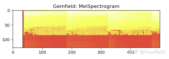
参数除了Spectrogram算法本来就需要的那些外,还多了:
- sample_rate,audio的采样率;
- n_mels,梅尔标度滤波器组的数量。
值得一提的是,苹果在wwdc上展示的傻瓜型的声音分类训练(用createML,Core ML 3中新增的功能)中使用的SoundAnalysisPreprocessing,就是将audio samples转换成了mel spectrograms。Gemfield从官方实现中(https://github.com/apple/coremltools/blob/master/mlmodel/format/SoundAnalysisPreprocessing.proto)摘录了如下的步骤:
message SoundAnalysisPreprocessing {
    /* Vggish preprocesses input audio samples and makes them ready to
       be fed to Vggish feature extractor.
       c.f. https://arxiv.org/pdf/1609.09430.pdf
       The preprocessing takes input a single channel (monophonic) audio samples
       975 miliseconds long, sampled at 16KHz, i.e., 15600 samples 1D multiarray
       and produces preprocessed samples in multiarray of shape [1, 96, 64]
     (1) Splits the input audio samples into overlapping frames, where each
         frame is 25 milliseconds long and hops forward by 10 milliseconds.
         Any partial frames at the end are dropped.
     (2) Hann window: apply a periodic Hann with a window_length of
         25 milliseconds, which translates to 400 samples in 16KHz sampling rate
         w(n) = 0.5 - 0.5 * cos(2*pi*n/window_length_sample),
         where 0 <= n <= window_lenth_samples - 1 and window_lenth_samples = 400
         Then, the Hann window is applied to each frame as below
         windowed_frame(n) = frame(n) * w(n)
         where 0 <= n <= window_lenth_samples - 1 and window_lenth_samples = 400
     (3) Power spectrum: calculate short-time Fourier transfor magnitude, with
         an FFT length of 512
     (4) Log Mel filter bank: calculates a log magnitude mel-frequency
         spectrogram minimum frequency of 125Hz and maximum frequency of 7500Hz,
         number of mel bins is 64, log_offset is 0.01, number of spectrum bins
         is 64.
    */
}可见使用了vggish项目的思路,在Vggish项目中(https://github.com/tensorflow/models/tree/master/research/audioset/vggish),audio的特征是按照如下步骤计算的:
- All audio is resampled to 16 kHz mono.
- A spectrogram is computed using magnitudes of the Short-Time Fourier Transform with a window size of 25 ms, a window hop of 10 ms, and a periodic Hann window.
- A mel spectrogram is computed by mapping the spectrogram to 64 mel bins covering the range 125-7500 Hz.
- A stabilized log mel spectrogram is computed by applying log(mel-spectrum + 0.01) where the offset is used to avoid taking a logarithm of zero.
- These features are then framed into non-overlapping examples of 0.96 seconds, where each example covers 64 mel bands and 96 frames of 10 ms each.
可见从torchaudio到CoreML3再到tensorflow,大家思路都一样。
4,其它算法
比如音频压缩类的(Mu-law算法,G.711中用到的)、有计算spectrogram的delta coefficients的(近似导数,比如torchaudio的compute_deltas,就是在声谱图视角下进行的计算)、滤波器类的(比如torchaudio functional中的highpass_biquad,高通滤波器)、特征类的(比如mfcc,essentia的mfcc是这么计算的:frame--> window --> spectrum --> mfcc,然后可以获取mfcc_bands和mfcc_coeffs,后者是一帧音频的前13个梅尔系数)。
以及其它多种多样的,比如essentia库中就包含了下面这么多知名不知名的算法:
AfterMaxToBeforeMaxEnergyRatio
AllPass
AutoCorrelation
BFCC
BPF
BandPass
BandReject
BarkBands
BeatTrackerDegara
BeatTrackerMultiFeature
Beatogram
BeatsLoudness
BinaryOperator
BinaryOperatorStream
BpmHistogram
BpmHistogramDescriptors
BpmRubato
CartesianToPolar
CentralMoments
Centroid
ChordsDescriptors
ChordsDetection
ChordsDetectionBeats
Chromagram
Clipper
ConstantQ
Crest
CrossCorrelation
CubicSpline
DCRemoval
DCT
Danceability
Decrease
Derivative
DerivativeSFX
Dissonance
DistributionShape
Duration
DynamicComplexity
ERBBands
EasyLoader
EffectiveDuration
Energy
EnergyBand
EnergyBandRatio
Entropy
Envelope
EqloudLoader
EqualLoudness
Extractor
FFT
FFTC
FadeDetection
Flatness
FlatnessDB
FlatnessSFX
Flux
FrameCutter
FrameGenerator
FrameToReal
FreesoundExtractor
FrequencyBands
GFCC
GeometricMean
HFC
HPCP
HarmonicBpm
HarmonicMask
HarmonicModelAnal
HarmonicPeaks
HighPass
HighResolutionFeatures
HprModelAnal
HpsModelAnal
IDCT
IFFT
IIR
Inharmonicity
InstantPower
Intensity
Key
KeyExtractor
LPC
Larm
Leq
LevelExtractor
LogAttackTime
LoopBpmConfidence
LoopBpmEstimator
Loudness
LoudnessEBUR128
LoudnessVickers
LowLevelSpectralEqloudExtractor
LowLevelSpectralExtractor
LowPass
MFCC
Magnitude
MaxFilter
MaxMagFreq
MaxToTotal
Mean
Median
MelBands
MetadataReader
Meter
MinToTotal
MonoLoader
MonoMixer
MonoWriter
MovingAverage
MultiPitchKlapuri
MultiPitchMelodia
Multiplexer
MusicExtractor
NoiseAdder
NoveltyCurve
NoveltyCurveFixedBpmEstimator
OddToEvenHarmonicEnergyRatio
OnsetDetection
OnsetDetectionGlobal
OnsetRate
Onsets
OverlapAdd
PCA
Panning
PeakDetection
PercivalBpmEstimator
PercivalEnhanceHarmonics
PercivalEvaluatePulseTrains
PitchContourSegmentation
PitchContours
PitchContoursMelody
PitchContoursMonoMelody
PitchContoursMultiMelody
PitchFilter
PitchMelodia
PitchSalience
PitchSalienceFunction
PitchSalienceFunctionPeaks
PitchYin
PitchYinFFT
PolarToCartesian
PoolAggregator
PowerMean
PowerSpectrum
PredominantPitchMelodia
RMS
RawMoments
ReplayGain
Resample
ResampleFFT
RhythmDescriptors
RhythmExtractor
RhythmExtractor2013
RhythmTransform
RollOff
SBic
Scale
SilenceRate
SineModelAnal
SineModelSynth
SineSubtraction
SingleBeatLoudness
SingleGaussian
Slicer
SpectralCentroidTime
SpectralComplexity
SpectralContrast
SpectralPeaks
SpectralWhitening
Spectrum
SpectrumCQ
SpectrumToCent
Spline
SprModelAnal
SprModelSynth
SpsModelAnal
SpsModelSynth
StartStopSilence
StereoDemuxer
StereoMuxer
StereoTrimmer
StochasticModelAnal
StochasticModelSynth
StrongDecay
StrongPeak
SuperFluxExtractor
SuperFluxNovelty
SuperFluxPeaks
TCToTotal
TempoScaleBands
TempoTap
TempoTapDegara
TempoTapMaxAgreement
TempoTapTicks
TonalExtractor
TonicIndianArtMusic
TriangularBands
TriangularBarkBands
Trimmer
Tristimulus
TuningFrequency
TuningFrequencyExtractor
UnaryOperator
UnaryOperatorStream
Variance
Vibrato
WarpedAutoCorrelation
Windowing
ZeroCrossingRate音乐信息检索MIR
音乐占据声音研究中的一大比例。当声音是音乐时,这个领域人们一般研究的话题就是和音乐相关了,比如Essentia库中的一个常用的类就是MusicExtractor。这个领域称之为音乐信息检索(MIR)。下面Gemfield列举了音乐方面一些常见的研究领域。
1,音乐节拍点
获得音乐节拍点的算法已经比较成熟了,但是,要想进一步获得强拍点还是弱拍点(也就是downbeat还是upbeat),目前的算法还做不到。在essentia中,可以使用
from essentia.standard import *

# Loading audio file
audio = MonoLoader(filename='gemfield_dubstep.flac')()

# Compute beat positions and BPM
rhythm_extractor = RhythmExtractor2013(method="multifeature")
bpm, beats, beats_confidence, _, beats_intervals = rhythm_extractor(audio)

print("BPM:", bpm)
print("Beat positions (sec.):", beats)
print("Beat estimation confidence:", beats_confidence)
可以得到每分钟的节拍数量、节拍的位置等。BPM还可以继续通过BpmHistogramDescriptors得到BPM的直方图,如果音乐节拍忽快忽慢的话,这个指标就很有意义了。
2,音符起始点检测(Onset detection)
essentia的OnsetDetection提供了多种算法,比如hfc、complex等。
# Loading audio file
audio = MonoLoader(filename='gemfield_hiphop.mp3')()

# Phase 1: compute the onset detection function
# The OnsetDetection algorithm provides various onset detection functions. Let's use two of them.

od1 = OnsetDetection(method='hfc')
od2 = OnsetDetection(method='complex')

# Let's also get the other algorithms we will need, and a pool to store the results
w = Windowing(type = 'hann')
fft = FFT() # this gives us a complex FFT
c2p = CartesianToPolar() # and this turns it into a pair (magnitude, phase)
pool = essentia.Pool()

# Computing onset detection functions.
for frame in FrameGenerator(audio, frameSize = 1024, hopSize = 512):
    mag, phase, = c2p(fft(w(frame)))
    pool.add('features.hfc', od1(mag, phase))
    pool.add('features.complex', od2(mag, phase))

# Phase 2: compute the actual onsets locations
onsets = Onsets()

onsets_hfc = onsets(# this algo expects a matrix, not a vector
                    essentia.array([ pool['features.hfc'] ]),

                    # you need to specify weights, but as there is only a single
                    # function, it doesn't actually matter which weight you give it
                    [ 1 ])

onsets_complex = onsets(essentia.array([ pool['features.complex'] ]), [ 1 ])
3,旋律检测 Melody detection
检测一个音频文件中主要的旋律的音高,在essentia中,我们可以使用PredominantPitchMelodia算法,这个算法会对输入的audio进行旋律的检测,然后给出每个时间段上主要旋律瞬时的音高(单位Hz):
import numpy

# Load audio file; it is recommended to apply equal-loudness filter for PredominantPitchMelodia
loader = EqloudLoader(filename='gemfield.wav', sampleRate=44100)
audio = loader()
print("Duration of the audio sample [sec]:")
print(len(audio)/44100.0)

# Extract the pitch curve
# PitchMelodia takes the entire audio signal as input (no frame-wise processing is required)

pitch_extractor = PredominantPitchMelodia(frameSize=2048, hopSize=128)
pitch_values, pitch_confidence = pitch_extractor(audio)

# Pitch is estimated on frames. Compute frame time positions
pitch_times = numpy.linspace(0.0,len(audio)/44100.0,len(pitch_values)
4,音调分析(Tonality analysis)
就是分析音乐的调性,比如C大调、d小调等。这又是什么意思呢?Gemfield找来一篇解释,还是很通俗易懂的,来自知乎上的 https://www.zhihu.com/question/28481469/answer/79850430 :
大家都知道12345671(do re mi)是一个八度,八个音,七个音差。但每两个音之间的差距不是平均的。
两个do之间,不包括高音do,可以分成12份,每份是半音,两个半音是一个全音,这叫12平均律(等比平均)。
调式是7个主音之间一种结构关系,就是怎样在八度区间内分配12个半音,定义12345671。
大调是这样,全全半全全全半,加起来12个半音,对应12345671,do Re 之间差一个全音,
re mi全音,mi fa半音,以此类推后面都是全音直到xi do又是一个半音。我们一般从小唱的do Re mi就是这样。
那么什么是C大调,D大调等。C D E F G A B C是五线谱上代表音高的音符。每一个可以对应一个声音频率,即音高。
以中音C为例,调琴标准频率260赫兹左右(非准确值),即琴弦或簧片每秒震动260次发出的声波。
高八度的C就翻倍到520赫兹,八度就是频率加倍,在中间分12份就得到其他音阶。C大调就是以C,260赫兹,
为do的12345671,全全半全全全半,对应CDEFGABC。这样就可以算出DEF等的频率。D大调就是从D,
即C大调的2,开始的大调,音阶结构一样。比如同一首歌,男中音可以唱C大调,女高音可以用D大调,听起来调子一样,音高不同。
小调就是另外一种结构,全半全全半全全,同样以C开头的就是C小调。在键盘上就是CDd#FGg#a#C。
仍然是C到C,八度。如果还唱1234567,调子听起来却像大调的6712345(音高不同)。
“#”,读sharp,计算机语言C#也来源于此。
使用essentia库的HPCP、 key 和 scale算法(判断大调还是小调),可以根据输入的音乐得到类似“A minor“的结果。
5,指纹算法
音乐领域的一个常见应用就是,输入一段音乐旋律,然后提取指纹特征,然后把指纹特征送到数据库,查找该音乐的其它相关资料。
在essentia库中,Chromaprint接口封装了Chromaprint算法(提取chroma特征),可以使用这个接口来提取音乐的指纹:
# the specified file is not provided with this notebook, try using your own music instead
audio = es.MonoLoader(filename='Desakato-Tiempo de cobardes.mp3', sampleRate=44100)()
fingerprint = es.Chromaprinter()(audio)

client = 'hGU_Gmo7vAY' # This is not a valid key. Use your key.
duration = len(audio) / 44100.

# Composing a query asking for the fields: recordings, releasegroups and compress.
query = 'http://api.acoustid.org/v2/lookup?client=%s&meta=recordings+releasegroups+compress&duration=%i&fingerprint=%s' \
%(client, duration, fingerprint)

from six.moves import urllib
page = urllib.request.urlopen(query)
print(page.read())
6,歌曲的相似度比较
翻唱歌曲识别Cover song identification (CSI),用来看一首歌是不是抄袭或者翻唱了另外一首歌。这里用到了essentia库中的HPCP、ChromaCrossSimilarity、CoverSongSimilarity算法。Essentia库在这个方面还是很强的。
总结
音频领域特征工程化方面,Gemfield使用最多的库就是torchaudio、librosa、essentia。这些库提供的算法都是有关audio的,有很多的相似性。其中torchaudio没有关于音乐MIR方面的,而librosa和essentia都有涉及MIR。Essentia库的另一个特点就是支持了跨平台(甚至包含了移动端)。