LBP特征描述算子-人脸检测
1. 原理
| 进展 | 原始的LBP算子 | 圆形LBP算子 | 旋转不变性的 LBP 算子 | LBP等价模式 |
|---|---|---|---|---|
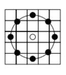
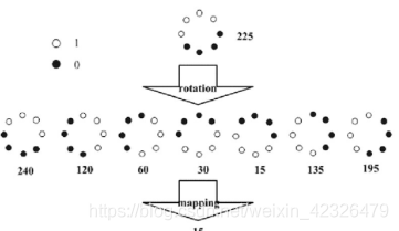
| 定义 | 在3*3的窗口内,以窗口中心像素为阈值,将相邻的8个像素的灰度值与其进行比较,若周围像素值大于中心像素值,则该像素点的位置被标记为1,否则为0 | 将 3×3 邻域扩展到任意邻域,并用圆形邻域代替了正方形邻域,改进后的 LBP 算子允许在半径为 R 的圆形邻域内有任意多个像素点 | 通过不断旋转圆形邻域得到一系列初始定义的 LBP 值,取其最小值作为该邻域的 LBP 值 | 当某个LBP所对应的循环二进制数从0到1或从1到0最多有两次跳变时,该LBP所对应的二进制就称为一个等价模式类 |
| 图示 | 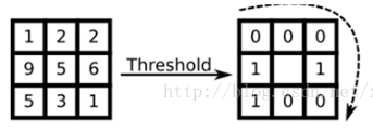 |
 |
 |
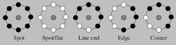 |
| 优点 | 具有灰度不变性 | 满足不同尺寸和频率纹理的需要 | 具有旋转不变性 | 解决了二进制模式过多的问题 |
2. LBP实现特征学习
2.1 步骤
- 首先将检测窗口划分为16×16的小区域(cell);
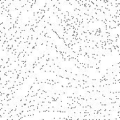
- 对于每个cell中的一个像素,将相邻的8个像素的灰度值与其进行比较,若周围像素值大于中心像素值,则该像素点的位置被标记为1,否则为0。这样,3*3邻域内的8个点经比较可产生8位二进制数,即得到该窗口中心像素点的LBP值;
- 然后计算每个cell的直方图,即每个数字(假定是十进制数LBP值)出现的频率;然后对该直方图进行归一化处理。
- 最后将得到的每个cell的统计直方图进行连接成为一个特征向量,也就是整幅图的LBP纹理特征向量;
- 最后便可利用SVM或者其他机器学习算法进行分类了。
2.2 代码
数据集的地址:https://pan.baidu.com/s/1bpjC7Vp
参考:https://blog.csdn.net/selous/article/details/69486823
import numpy as np
import matplotlib.image as mpimg
import matplotlib.pyplot as plt
from sklearn.multiclass import OneVsRestClassifier
from sklearn.svm import SVR
from skimage import feature as skft
import cv2
def loadPicture():
train_index = 0
test_index = 0
train_data = np.zeros( (200,171,171) )
test_data = np.zeros( (160,171,171) )
train_label = np.zeros( (200) )
test_label = np.zeros( (160) )
for i in np.arange(40):
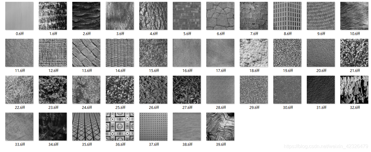
image = mpimg.imread('D:/python_opencv/picture/'+str(i)+'.tiff')
data = np.zeros( (513,513) )
data[0:image.shape[0],0:image.shape[1]] = image
#切割后的图像位于数据的位置
index = 0
#将图片分割成九块
for row in np.arange(3):
for col in np.arange(3):
if index<5:
train_data[train_index,:,:] = data[171*row:171*(row+1),171*col:171*(col+1)]
train_label[train_index] = i
train_index+=1
else:
test_data[test_index,:,:] = data[171*row:171*(row+1),171*col:171*(col+1)]
test_label[test_index] = i
test_index+=1
index+=1
return train_data,test_data,train_label,test_label
radius = 1
n_point = radius * 8
def texture_detect():
train_hist = np.zeros( (200,256) )
test_hist = np.zeros( (160,256) )
for i in np.arange(200):
#使用LBP方法提取图像的纹理特征.
lbp=skft.local_binary_pattern(train_data[i],n_point,radius,'default')
cv2.imshow("lbp",lbp)
#统计图像的直方图
max_bins = int(lbp.max() + 1)
#hist size:256
train_hist[i], _ = np.histogram(lbp, normed=True, bins=max_bins, range=(0, max_bins))
for i in np.arange(160):
lbp = skft.local_binary_pattern(test_data[i],n_point,radius,'default')
#统计图像的直方图
max_bins = int(lbp.max() + 1)
#hist size:256
test_hist[i], _ = np.histogram(lbp, normed=True, bins=max_bins, range=(0, max_bins))
return train_hist,test_hist
train_data,test_data,train_label,test_label= loadPicture()
train_hist,test_hist = texture_detect()
svr_rbf = SVR(kernel='rbf', C=1e3, gamma=0.1)
a = OneVsRestClassifier(svr_rbf,-1).fit(train_hist,
train_label).score(test_hist,test_label)
print(a)
#cv2.imshow("train_hist",test_hist)
2.3 特征学习成果
原始数据:
训练成果: