MF vs MLP

作者：九羽，炼丹笔记小编

文章目录

MF vs MLP

基于Embedding的推荐算法模型一直是近几年研究的热门，在各大国际会议期刊都能看到来自工业界研究与实践的成果。MF（Matrix Factorization）作为传统基于点积和高阶组合Embedding的方式，在推荐系统被广泛应用。对user和item的交互行为的建模大多使用MF，对user和item的隐特征使用内积计算，而这是一种线性方式。

而通过引入user、item偏置提高MF效果也说明内积不足以捕捉到用户交互数据中的复杂结构信息。因此在NCF（Neural Collaborative Filtering）论文中，作者引入深度学习方法对特征之间的相互关系进行非线性的描述是解决该问题的一种方式。

本文主要阐述的内容主要为：

1、在相同实验情况下，矩阵分解（Matrix Factorization）在进行参数调优之后是否能比MLP（Multi Layer Perceptron）具有较大幅度的提升？

2、虽然MLP理论上可以逼近任何函数，但是本文通过实验对比分析MLP与点积函数之间的逼近关系；

3、最后，讨论MLP在实际线上生成环境中提供Service时的高成本问题，对比“点积”可以通过类似Faiss等高效搜索算法快速找到相似Item。

什么是Dot Product 和MLP？

内积和MLP

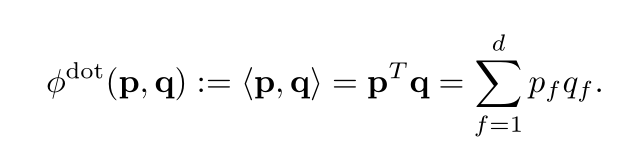
Dot Product

用户向量UserEmbedding（图中p）和物品向量ItemEmbedding（图中q）的点积。
在这里插入图片描述

MLP （Multi Layer Perceptron）& NCF

MLP理论上能拟合任何函数，在NCF论文中作者用MLP替换点积，将用户向量UserEmbedding和物品向量ItemEmbedding拼接后作为输入。

在这里插入图片描述

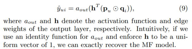
NCF网络可以分解为两个子网络，一个被称为广义矩阵分解Generalized Matrix Factorization (GMF)，另一个是多层感知机Multi-Layer Perceptron (MLP)。

其中GMF，利用用户向量UserEmbedding和物品向量ItemEmbedding，使用了哈达玛乘积进行组合（元素级别——相同大小的两个矩阵中对应位置元素相乘例如：(3x3)⊙(3x3) = 3x3），然后在全连接层进行了线性的加权组合，即训练了一个h向量(权重向量)。

MLP部分，用户向量UserEmbedding和物品向量ItemEmbedding进行拼接，然后输入多层FC层。由于<User，Item>的拼接操作后过FC层，所以这些特征经过了充分的非线性组合，最后的输出再使用sigmoid函数。

原论文里模型效果如下：
在这里插入图片描述

Dot Product vs. MLP

本文有意思的地方是作者提出了一个疑问，MLP模型真的优于点积吗？

基于以上的介绍，我们会有一种潜在的认知，使用MLP替换点积可以增强模型的表达能力，毕竟MLP具有拟合任意函数的能力。在《Neural Collaborative Filtering vs. Matrix Factorization Revisited》论文中，完成了对NCF实验的复现，同时在相同数据集上，采用留一法，保留每个用户最后一次点击作为验证。并且通过HR和NDCG评估点积Dot Product和NCF的效果如下：

通过图中的效果，是不是对原有的认知有所怀疑了。当然无论是原文中对比试验也好，还是本文想表达的，都不是否定Deep Learning推荐领域所发挥的积极作用。作为一名深度学习炼丹者，思考对比背后的一些意义反而更加有意思。原文中对调参部分的是较为详尽的，也是非常值得学习的，作者介绍了自己的炼丹过程，如何为矩阵分解（MF）模型搜索最优参数。

矩阵分解炼丹过程

论文原文
From our past experience with matrix factorization models, if the other hyperparameters are chosen properly, then the larger the embedding dimension the better the quality – our experiments Figure 2 confirm this. For the other hyperparameters: learning rate and number of training epochs influence the convergence curves. Usually, the lower the learning rate, the better the quality but also the more epochs are needed. We set a computational budget of up to 256 epochs and search for the learning rate within this setting. In the first hyperparameter pass, we search a coarse grid of learning rates η ∈ {0.001, 0.003, 0.01} and number of negatives m = {4, 8, 16} while fixing the regularization to λ = 0. Then we did a search for regularization in {0.001, 0.003, 0.01} around the promising candidates. To speed up the search, these first coarse passes were done with 128 epochs and a fixed dimension of d = 64 (Movielens) and d = 128 (Pinterest). We did further refinements around the most promising values of learning rate, number of negatives and regularization using d = 128 and 256 epochs.

Throughout the experiments we initialize embeddings from a Gaussian distribution with standard deviation of 0.1; we tested some variation of the standard deviation but did not see much effect. The final hyperparameters for Movielens are: learning rate η = 0.002, number of negatives m = 8, regularization λ = 0.005, number of epochs 256. For Pinterest: learning rate η = 0.007, number of negative samples m = 10, regularization λ = 0.01, number of epochs 256.

炼丹笔记

（1）训练集、验证集、测试集划分，用户最后一次点击作为测试集，倒数第二次点击作为验证集正样本。

（2）超参调整。可调参数列表：

参数	含义
epochs	训练轮数
m	负采样率
η	SGD学习率
d	Embedding维度
std	初始化模型系数的（标准正态分布的）标准差
λ	正则化系数

（3）利用Grid Search调整学习率η ∈ {0.001, 0.003, 0.01}和负采样率m={4,8,16}进行第一层结果粗粒度选择，然后选择较优的结果对λ = {0.001, 0.003, 0.01}进行第二层结果进行细粒度选择。于此同时固定epochs、embedding维数、标准差。

（4）对训练轮数，负采样率等进行调优；

参考文献

1、《Neural Collaborative Filtering vs. Matrix Factorization Revisited》

https://arxiv.org/abs/2005.09683

Filtering vs. Matrix Factorization Revisited》