Pillow图像处理库

图像处理库

matplotlib.image

仅支持导入PNG格式的图像，且功能有限

PIL(Python Imaging Library)

• 功能丰富，简单应用
• 仅支持python2.x版本，且已经停止更新

Pillow

• 在PIL的基础上发展而成
• 支持python3

安装和导入包/模块

• PIllow的安装
  • 使用Anaconda
  • 使用pip命令安装

pip install pillow

• 导入PIL.image模块
  通过image类的函数、方法和属性，完成对图像的读取、显示和简单的操作

from PIL import image

• 导入matplotlib.pyplot
  用来显示图片

import matplotlib.pyplot as plt

打开图像-image.open()函数

image.open(path)

返回image对象
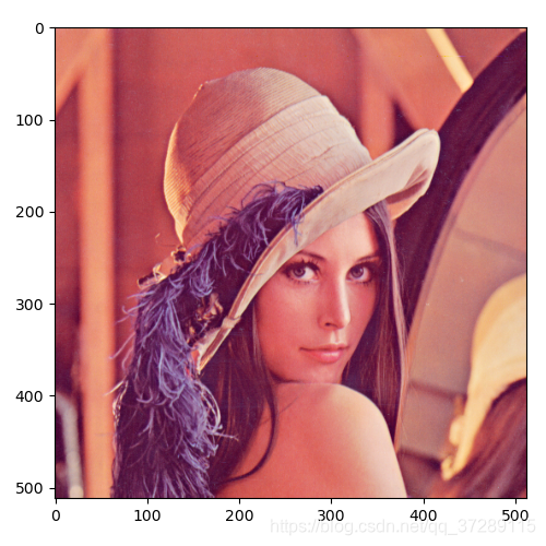
这是在数字图像处理中非常常用的图像Lena，下载Lena.tiff
然后将它复制到工作目录就可以使用了

保存图像-save()函数

图像对象.save(文件路径)
img.save("test.tiff")	# 将对象保存为test.tiff

还可以改变文件名的后缀，就可以转换图像格式

img.save("lena.jpg")
img.save("lena.bmp")

图像对象的主要属性

属性	说明
图像对象.format	图像格式
图像对象.size	图像尺寸
图像对象.mode	色彩模式

• 图像格式

img = Image.open("lena512color.tiff")
# img.save("test.tiff")
# img.save("lena.jpg")
# img.save("lena.bmp")

img1 = Image.open("lena.jpg")
img2 = Image.open("lena.bmp")

print("image:", img.format)
print("image1:", img1.format)
print("image2:", img2.format)

运行结果

• 尺寸和色彩模式

print("image:", img.size)
print("image:", img.mode)

运行结果

显示图像

imshow()

plt.imshow(image对象/Numpy数组)

show()

import matplotlib.pyplot as plt
plt.figure(figsize=(5, 5))
plt.imshow(img)
plt.show()

运行结果

下面我们分别显示不同类型的图像

plt.figure(figsize=(15, 5))

plt.subplot(131)
plt.axis("off")
plt.imshow(img)
plt.title(img.format)

plt.subplot(132)
plt.axis("off")
plt.imshow(img)
plt.title(img1.format)

plt.subplot(133)
plt.axis("off")
plt.imshow(img)
plt.title(img2.format)

plt.show()

运行结果

转换图像的色彩模式

取值	色彩模式
1	二值图像
L	灰度图像
P	8位彩色图像
RGB	24位彩色图像
RGBA	32位彩色图像
CMYK	CMYK彩色图像
YCbCr	YCbCr彩色图像
l	32位整型灰度图像
F	32位浮点灰度图像

图像对象.convert(色彩模式)

img_gray = img.convert("L")
print("mode=", img_gray.mode)
plt.figure(figsize=(5, 5))
plt.imshow(img_gray)
plt.show()

也可以通过save()来保存这个灰度图像

img_gray.save("lena_gray.bmp")

运行结果

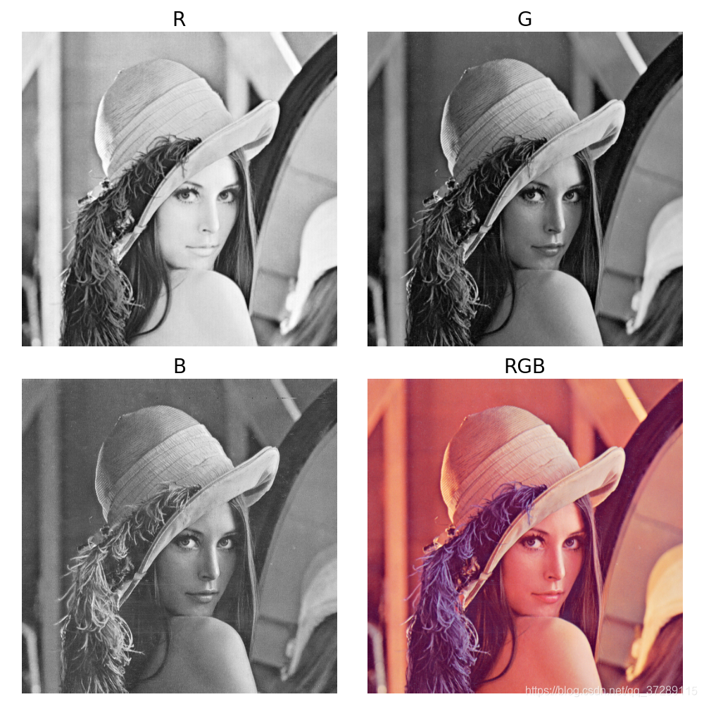
颜色通道的分离与合并

可以使用split方法 将彩色图片的各个通道分离出来

图像对象.split()

用merge方法，将通道合并起来

Image.merge(色彩模式, 图像列表)

img = Image.open("lena512color.tiff")
img_r, img_g, img_b = img.split()
plt.figure(figsize=(10, 10))

plt.subplot(221)
plt.axis("off")
plt.imshow(img_r, cmap="gray")
plt.title("R", fontsize=20)

plt.subplot(222)
plt.axis("off")
plt.imshow(img_g, cmap="gray")
plt.title("G", fontsize=20)

plt.subplot(223)
plt.axis("off")
plt.imshow(img_b, cmap="gray")
plt.title("B", fontsize=20)

img_rbg = Image.merge("RGB", [img_r, img_g, img_b])
plt.subplot(224)
plt.axis("off")
plt.imshow(img_rbg, cmap="gray")
plt.title("RGB", fontsize=20)

plt.show()

运行结果

转化为数组

np.array(图像对象)

import numpy as np
arr_img = np.array(img)
print("shape=", arr_img.shape)
print(arr_img)

运行结果

shape= (512, 512, 3)
[[[226 137 125]
  [226 137 125]
  [223 137 133]
  ...
  [230 148 122]
  [221 130 110]
  [200  99  90]]
 [[226 137 125]
  [226 137 125]
  [223 137 133]
  ...
  [230 148 122]
  [221 130 110]
  [200  99  90]]
 [[226 137 125]
  [226 137 125]
  [223 137 133]
  ...
  [230 148 122]
  [221 130 110]
  [200  99  90]]
 ...
 [[ 84  18  60]
  [ 84  18  60]
  [ 92  27  58]
  ...
  [173  73  84]
  [172  68  76]
  [177  62  79]]
 [[ 82  22  57]
  [ 82  22  57]
  [ 96  32  62]
  ...
  [179  70  79]
  [181  71  81]
  [185  74  81]]
 [[ 82  22  57]
  [ 82  22  57]
  [ 96  32  62]
  ...
  [179  70  79]
  [181  71  81]
  [185  74  81]]]

图像对象是一个三维数组，前两维对应图像的尺寸，第三维对应它的通道。

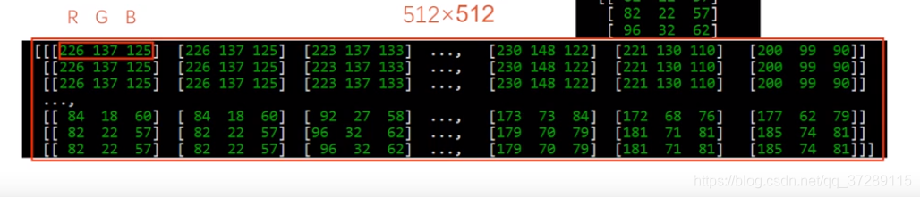
每一个元素对应图像的像素。

将灰度图像lena_gray.bmp转化为数组

img_gray = Image.open("lena_gray.bmp")
arr_img_gray = np.array(img_gray)
print("\nshape:", arr_img_gray.shape)
print(arr_img_gray)

运行结果

shape: (512, 512)
[[162 162 162 ... 170 155 128]
 [162 162 162 ... 170 155 128]
 [162 162 162 ... 170 155 128]
 ...
 [ 43  43  50 ... 104 100  98]
 [ 44  44  55 ... 104 105 108]
 [ 44  44  55 ... 104 105 108]]

可以看到，这是一个512*512的二维数组，其中每个元素对应一个像素。现在这个图像已经是一个numpy数组了，可以对它进行任意处理。比如反色处理。

img_gray = Image.open("lena_gray.bmp")
arr_img_gray = np.array(img_gray)
print("\nshape:", arr_img_gray.shape)
print(arr_img_gray)

arr_img_new = 255 - arr_img_gray    # 对图像中每一个像素进行反色处理
plt.figure(figsize=(10, 5))

plt.subplot(121)
plt.axis("off")
plt.imshow(arr_img_gray, cmap="gray")

plt.subplot(122)
plt.axis("off")
plt.imshow(arr_img_new, cmap="gray")

plt.show()

对图像的缩放、旋转和镜像

Image模块中还提供了很多封装好了的函数，可以直接对图片进行更上乘的处理，而不用将图片转化成数组

• 缩放图像

图像对象.resize((width, height))

img = Image.open("lena512color.tiff")
plt.figure(figsize=(5, 5))
img_small = img.resize((64, 64))

plt.imshow(img_small)
plt.show()
img_small.save("lena_s.jpg")

运行结果

可以看到图片的质量明显下降了，出现了马赛克的效应。通过坐标轴可以发现图片的像素尺寸变成了64*64，这是个降采样的过程。

可以看到这个图像是原图像的四分之一。

图像对象.thummbnail((width, height))

这也是缩放图片，但这个是原地操作，返回值是None。也就是说直接对image对象进行了缩放。

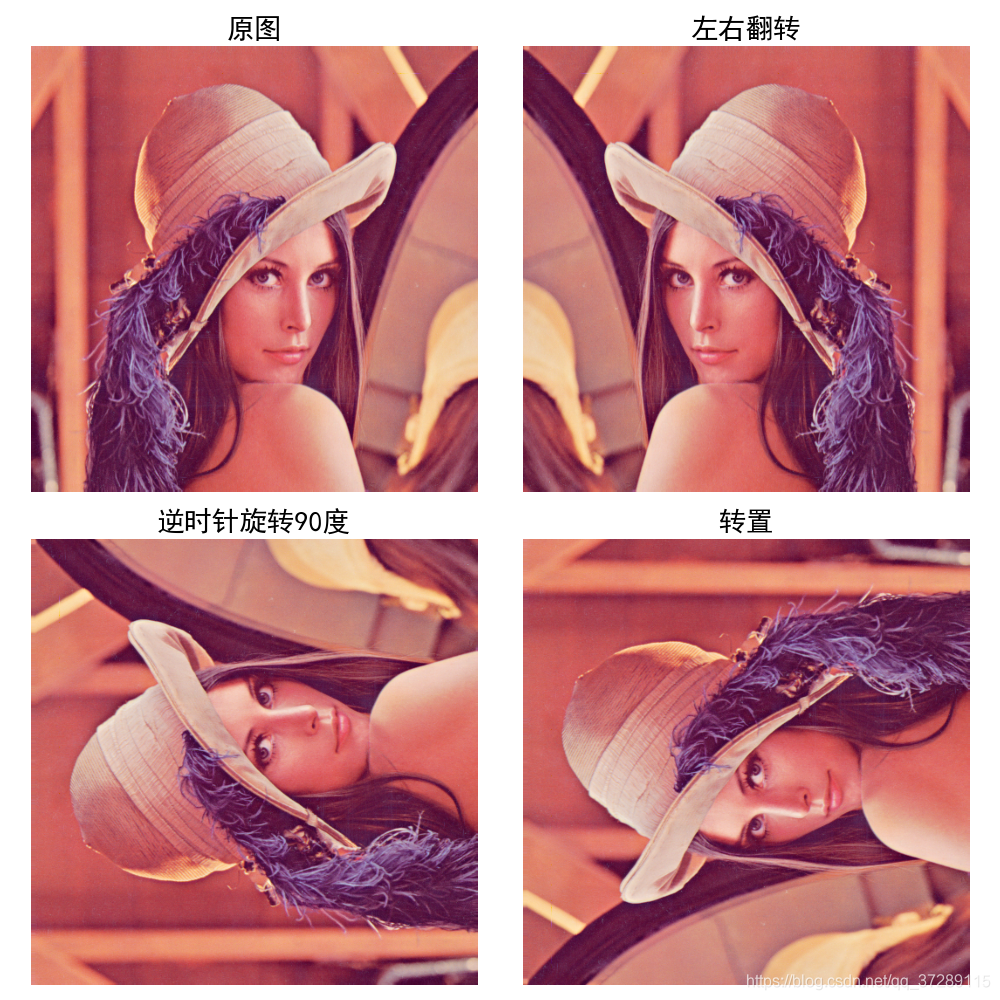
• 旋转、镜像

图像对象.transpose(旋转方式)

Image.FLIP_LEFT_RIGHT：水平翻转
Image.FLIP_TOP_BOTTOM：上下翻转
Image.ROTATE_90：逆时针翻转90度
Image.ROTATE_180：逆时针翻转180度
Image.ROTATE_270：逆时针翻转270度
Image.TRANSPOSE：将图像进行转置
Image.TRANSVERSE：将图像进行转置，再水平翻转

img_flr = img.transpose(Image.FLIP_LEFT_RIGHT)
img_r90 = img.transpose(Image.ROTATE_90)
img_tp = img.transpose(Image.TRANSPOSE)

下面我们将变换的结果分别显示在不同的子图中。

plt.rcParams['font.sans-serif'] = "SimHei"
img = Image.open("lena512color.tiff")

plt.figure(figsize=(10, 10))

plt.subplot(221)
plt.axis("off")
plt.imshow(img)
plt.title("原图", fontsize=20)

plt.subplot(222)
plt.axis("off")
img_flr = img.transpose(Image.FLIP_LEFT_RIGHT)
plt.imshow(img_flr)
plt.title("左右翻转", fontsize=20)

plt.subplot(223)
plt.axis("off")
img_r90 = img.transpose(Image.ROTATE_90)
plt.imshow(img_r90)
plt.title("逆时针旋转90度", fontsize=20)

plt.subplot(224)
plt.axis("off")
img_tp = img.transpose(Image.TRANSPOSE)
plt.imshow(img_tp)
plt.title("转置", fontsize=20)

plt.show()

运行结果

• 裁剪图像：在图像上指定的位置裁剪出一个矩形区域

图像对象.crop((x0, y0, x1, y1))

其中$x_0$和$y_0$是左上角坐标，$x_1$和$y_1$是右下角坐标，坐标的单位是像素。
返回值：图像对象

img = Image.open("lena512color.tiff")

plt.figure(figsize=(10, 5))

plt.subplot(121)
plt.imshow(img)

plt.subplot(122)
img_region = img.crop((100, 100, 400, 400))
plt.imshow(img_region)

plt.show()