在pandas中创建图像
import pandas as pd
import matplotlib.pyplot as plt
1. 使用空气质量数据air_quality_no2.csv
air_quality=pd.read_csv("data/air_quality_no2.csv",index_col=0,parse_dates=True)
air_quality.head()
#index_col=0,parse_dates=True表示把返回的表格的第一列作为索引,
#把列中的数组转化为Timestamp
| station_antwerp | station_paris | station_london | |
|---|---|---|---|
| datetime | |||
| 2019-05-07 02:00:00 | NaN | NaN | 23.0 |
| 2019-05-07 03:00:00 | 50.5 | 25.0 | 19.0 |
| 2019-05-07 04:00:00 | 45.0 | 27.7 | 19.0 |
| 2019-05-07 05:00:00 | NaN | 50.4 | 16.0 |
| 2019-05-07 06:00:00 | NaN | 61.9 | NaN |
2. 可视化数据
plt.plot(air_quality)
[<matplotlib.lines.Line2D at 0x227a8689488>,
 <matplotlib.lines.Line2D at 0x227a91e7608>,
 <matplotlib.lines.Line2D at 0x227a91e7688>]
air_quality.plot()
<matplotlib.axes._subplots.AxesSubplot at 0x227a80e86c8>

2. visually compare the N02 values measured in London versus Paris.
air_quality.plot.scatter(x="station_london",y="station_paris",alpha=0.5)#alpha表示透明度
<matplotlib.axes._subplots.AxesSubplot at 0x227ab575848>

plt.scatter(air_quality["station_london"],air_quality["station_paris"] ,alpha=0.2)
<matplotlib.collections.PathCollection at 0x227a96d3388>

3.一些标准的Python来概述可用的绘图方法:
[method_name for method_name in dir(air_quality.plot) if not method_name.startswith("_")]
['area',
 'bar',
 'barh',
 'box',
 'density',
 'hexbin',
 'hist',
 'kde',
 'line',
 'pie',
 'scatter']
注意
在许多开发环境比如ipython和jupyter nootbook,请使用TAB按钮获得全部的可用方法,例如air_quality.plot.+ TAB。
air_quality.plot.box()
<matplotlib.axes._subplots.AxesSubplot at 0x227ac9382c8>

4.每个列在单独的子图中:subplots
axs=air_quality.plot.area(figsize=(12,4),subplots=True)

5.进一步自定义,扩展或保存生成的图。
fig, axs = plt.subplots(figsize=(12, 4))        # Create an empty matplotlib Figure and Axes
air_quality.plot.area(ax=axs)                   # Use pandas to put the area plot on the prepared Figure/Axes
axs.set_ylabel("NO$_2$ concentration")          # Do any matplotlib customization you like
fig.savefig("no2_concentrations.png")           # Save the Figure/Axes using the existing matplotlib method.

小结:
-
该.plot.*方法适用于Series和DataFrames
-
默认情况下,每个列都用不同的元素(线,箱线图等)绘制
-
pandas创建的任何plot都是Matplotlib对象。
扫描二维码关注公众号,回复: 11628347 查看本文章
从现有列派生出新的列
#表达 NO2 伦敦车站的浓度,mg / m3
#(如果我们假设温度为25摄氏度,压力为1013 hPa,则转换因子为1.882)

air_quality["londom-mg_per_cubic"]=air_quality["station_london"]*1.882
air_quality.head()
| station_antwerp | station_paris | station_london | londom-mg_per_cubic | |
|---|---|---|---|---|
| datetime | ||||
| 2019-05-07 02:00:00 | NaN | NaN | 23.0 | 43.286 |
| 2019-05-07 03:00:00 | 50.5 | 25.0 | 19.0 | 35.758 |
| 2019-05-07 04:00:00 | 45.0 | 27.7 | 19.0 | 35.758 |
| 2019-05-07 05:00:00 | NaN | 50.4 | 16.0 | 30.112 |
| 2019-05-07 06:00:00 | NaN | 61.9 | NaN | NaN |
#求巴黎与安特卫普的值之比,并将结果保存在新列中
air_quality["ratio_paris_anwerp"]=air_quality["station_paris"]/air_quality["station_antwerp"]
air_quality.head()
| station_antwerp | station_paris | station_london | londom-mg_per_cubic | ratio_paris_anwerp | |
|---|---|---|---|---|---|
| datetime | |||||
| 2019-05-07 02:00:00 | NaN | NaN | 23.0 | 43.286 | NaN |
| 2019-05-07 03:00:00 | 50.5 | 25.0 | 19.0 | 35.758 | 0.495050 |
| 2019-05-07 04:00:00 | 45.0 | 27.7 | 19.0 | 35.758 | 0.615556 |
| 2019-05-07 05:00:00 | NaN | 50.4 | 16.0 | 30.112 | NaN |
| 2019-05-07 06:00:00 | NaN | 61.9 | NaN | NaN | NaN |
rename()
- 可用于行标签和列标签。
- 提供一个字典,其中包含键,当前名称和值,以及新名称.
#将数据列重命名为openAQ使用的相应工作站标识符werp
air_quality_renamed=air_quality.rename(columns={
    "station_anterp":"BETR801",
    "staion_paris":"FR04014",
    "staion_london":"London Westminster"})
air_quality_renamed.head()
| station_antwerp | station_paris | station_london | londom-mg_per_cubic | ratio_paris_anwerp | |
|---|---|---|---|---|---|
| datetime | |||||
| 2019-05-07 02:00:00 | NaN | NaN | 23.0 | 43.286 | NaN |
| 2019-05-07 03:00:00 | 50.5 | 25.0 | 19.0 | 35.758 | 0.495050 |
| 2019-05-07 04:00:00 | 45.0 | 27.7 | 19.0 | 35.758 | 0.615556 |
| 2019-05-07 05:00:00 | NaN | 50.4 | 16.0 | 30.112 | NaN |
| 2019-05-07 06:00:00 | NaN | 61.9 | NaN | NaN | NaN |
# rename()映射不仅应限于固定名称,还可以是映射函数

air_quality_renamed=air_quality.rename(columns=str.lower)#将列名转为小写
air_quality_renamed.head()
| station_antwerp | station_paris | station_london | londom-mg_per_cubic | ratio_paris_anwerp | |
|---|---|---|---|---|---|
| datetime | |||||
| 2019-05-07 02:00:00 | NaN | NaN | 23.0 | 43.286 | NaN |
| 2019-05-07 03:00:00 | 50.5 | 25.0 | 19.0 | 35.758 | 0.495050 |
| 2019-05-07 04:00:00 | 45.0 | 27.7 | 19.0 | 35.758 | 0.615556 |
| 2019-05-07 05:00:00 | NaN | 50.4 | 16.0 | 30.112 | NaN |
| 2019-05-07 06:00:00 | NaN | 61.9 | NaN | NaN | NaN |
小结:
-
创建新列:把基于现有列的计算结果赋值给[]中的新列名。
-
操作是基于元素的,不需要遍历行。
-
rename与字典或函数一起使用来重命名行标签或列名。
计算汇总统计信息
titanic=pd.read_csv("data/titanic.csv")
titanic.head()
| PassengerId | Survived | Pclass | Name | Sex | Age | SibSp | Parch | Ticket | Fare | Cabin | Embarked | |
|---|---|---|---|---|---|---|---|---|---|---|---|---|
| 0 | 1 | 0 | 3 | Braund, Mr. Owen Harris | male | 22.0 | 1 | 0 | A/5 21171 | 7.2500 | NaN | S |
| 1 | 2 | 1 | 1 | Cumings, Mrs. John Bradley (Florence Briggs Th... | female | 38.0 | 1 | 0 | PC 17599 | 71.2833 | C85 | C |
| 2 | 3 | 1 | 3 | Heikkinen, Miss. Laina | female | 26.0 | 0 | 0 | STON/O2. 3101282 | 7.9250 | NaN | S |
| 3 | 4 | 1 | 1 | Futrelle, Mrs. Jacques Heath (Lily May Peel) | female | 35.0 | 1 | 0 | 113803 | 53.1000 | C123 | S |
| 4 | 5 | 0 | 3 | Allen, Mr. William Henry | male | 35.0 | 0 | 0 | 373450 | 8.0500 | NaN | S |
1.平均数
#泰坦尼克号旅客的平均年龄
titanic["Age"].mean()
29.69911764705882
2. 中位数
titanic[["Age","Fare"]].median()
Age     28.0000
Fare    14.4542
dtype: float64
titanic[["Age","Fare"]].describe()
| Age | Fare | |
|---|---|---|
| count | 714.000000 | 891.000000 |
| mean | 29.699118 | 32.204208 |
| std | 14.526497 | 49.693429 |
| min | 0.420000 | 0.000000 |
| 25% | 20.125000 | 7.910400 |
| 50% | 28.000000 | 14.454200 |
| 75% | 38.000000 | 31.000000 |
| max | 80.000000 | 512.329200 |
3. DataFrame.agg()
使用指定轴上的一项或多项操作进行汇总
titanic.agg({'Age':['min','max','median','skew'],
             'Fare':['min','max','median','mean']})
| Age | Fare | |
|---|---|---|
| max | 80.000000 | 512.329200 |
| mean | NaN | 32.204208 |
| median | 28.000000 | 14.454200 |
| min | 0.420000 | 0.000000 |
| skew | 0.389108 | NaN |
4.groupby():按类别分组
- 获取按类别(属性)分组的统计信息
- 分组可以同时由多个列完成。提供列名作为groupby()方法的列表
#男性和女性泰坦尼克号乘客的平均年龄
titanic[["Sex","Age"]].groupby('Sex').mean()
| Age | |
|---|---|
| Sex | |
| female | 27.915709 |
| male | 30.726645 |
titanic.groupby('Sex').mean()
| PassengerId | Survived | Pclass | Age | SibSp | Parch | Fare | |
|---|---|---|---|---|---|---|---|
| Sex | |||||||
| female | 431.028662 | 0.742038 | 2.159236 | 27.915709 | 0.694268 | 0.649682 | 44.479818 |
| male | 454.147314 | 0.188908 | 2.389948 | 30.726645 | 0.429809 | 0.235702 | 25.523893 |
#我们只对每种性别的平均年龄感兴趣
titanic.groupby('Sex')['Age'].mean()
Sex
female    27.915709
male      30.726645
Name: Age, dtype: float64
#性别和客舱舱位组合的平均票价
titanic.groupby(['Sex','Pclass'])['Fare'].mean()
Sex     Pclass
female  1         106.125798
        2          21.970121
        3          16.118810
male    1          67.226127
        2          19.741782
        3          12.661633
Name: Fare, dtype: float64
5.value_counts():按类别统计数目
#每个舱位的乘客人数
titanic['Pclass'].value_counts()
3    491
1    216
2    184
Name: Pclass, dtype: int64
#它实际上是一个groupby操作,结合了对每个组中记录数的计数
titanic.groupby('Pclass')['Pclass'].count()
Pclass
1    216
2    184
3    491
Name: Pclass, dtype: int64
注意:
- size()和count()都可以和groupby()一起用
- size包括NaN(size of the table)
- count排除了缺省值
- value_counts()可以使用drapna()去增/去 Nan
小结:
-
可以对整列或整行计算聚合统计信息
-
groupby提供 拆分-应用-组合 模式的功能
-
value_counts 是一种方便的快捷方式,用于计算每个类别中的条目数
对表格进行重新布局
1. 对表格进行排序
- 使用.sort_values(),将根据定义的列对表中的行进行排序。索引将遵循行顺序。
 #根据乘客的年龄对泰坦尼克号数据进行排序。
titanic.sort_values(by='Age').head()
| PassengerId | Survived | Pclass | Name | Sex | Age | SibSp | Parch | Ticket | Fare | Cabin | Embarked | |
|---|---|---|---|---|---|---|---|---|---|---|---|---|
| 803 | 804 | 1 | 3 | Thomas, Master. Assad Alexander | male | 0.42 | 0 | 1 | 2625 | 8.5167 | NaN | C |
| 755 | 756 | 1 | 2 | Hamalainen, Master. Viljo | male | 0.67 | 1 | 1 | 250649 | 14.5000 | NaN | S |
| 644 | 645 | 1 | 3 | Baclini, Miss. Eugenie | female | 0.75 | 2 | 1 | 2666 | 19.2583 | NaN | C |
| 469 | 470 | 1 | 3 | Baclini, Miss. Helene Barbara | female | 0.75 | 2 | 1 | 2666 | 19.2583 | NaN | C |
| 78 | 79 | 1 | 2 | Caldwell, Master. Alden Gates | male | 0.83 | 0 | 2 | 248738 | 29.0000 | NaN | S |
#根据机舱等级和年龄按降序对泰坦尼克号数据进行排序
titanic.sort_values(by=["Pclass","Age"],ascending=False).head()
| PassengerId | Survived | Pclass | Name | Sex | Age | SibSp | Parch | Ticket | Fare | Cabin | Embarked | |
|---|---|---|---|---|---|---|---|---|---|---|---|---|
| 851 | 852 | 0 | 3 | Svensson, Mr. Johan | male | 74.0 | 0 | 0 | 347060 | 7.7750 | NaN | S |
| 116 | 117 | 0 | 3 | Connors, Mr. Patrick | male | 70.5 | 0 | 0 | 370369 | 7.7500 | NaN | Q |
| 280 | 281 | 0 | 3 | Duane, Mr. Frank | male | 65.0 | 0 | 0 | 336439 | 7.7500 | NaN | Q |
| 483 | 484 | 1 | 3 | Turkula, Mrs. (Hedwig) | female | 63.0 | 0 | 0 | 4134 | 9.5875 | NaN | S |
| 326 | 327 | 0 | 3 | Nysveen, Mr. Johan Hansen | male | 61.0 | 0 | 0 | 345364 | 6.2375 | NaN | S |
air_quality=pd.read_csv("data/air_quality_long.csv",index_col="date.utc",parse_dates=True)
air_quality.head()
| city | country | location | parameter | value | unit | |
|---|---|---|---|---|---|---|
| date.utc | ||||||
| 2019-06-18 06:00:00+00:00 | Antwerpen | BE | BETR801 | pm25 | 18.0 | µg/m³ |
| 2019-06-17 08:00:00+00:00 | Antwerpen | BE | BETR801 | pm25 | 6.5 | µg/m³ |
| 2019-06-17 07:00:00+00:00 | Antwerpen | BE | BETR801 | pm25 | 18.5 | µg/m³ |
| 2019-06-17 06:00:00+00:00 | Antwerpen | BE | BETR801 | pm25 | 16.0 | µg/m³ |
| 2019-06-17 05:00:00+00:00 | Antwerpen | BE | BETR801 | pm25 | 7.5 | µg/m³ |
2.长到宽表格式???Long to wide table format
[外链图片转存失败,源站可能有防盗链机制,建议将图片保存下来直接上传(img-MNKpTCte-1595753237357)(attachment:image.png)]
#过滤其他数据只要no2的数据
no2=air_quality[air_quality['parameter']=='no2']
#仅使用每个location(grouupby)的前两个测量值。
no2_subset=no2.sort_index().groupby("location").head(2)
no2_subset
| city | country | location | parameter | value | unit | |
|---|---|---|---|---|---|---|
| date.utc | ||||||
| 2019-04-09 01:00:00+00:00 | Antwerpen | BE | BETR801 | no2 | 22.5 | µg/m³ |
| 2019-04-09 01:00:00+00:00 | Paris | FR | FR04014 | no2 | 24.4 | µg/m³ |
| 2019-04-09 02:00:00+00:00 | London | GB | London Westminster | no2 | 67.0 | µg/m³ |
| 2019-04-09 02:00:00+00:00 | Antwerpen | BE | BETR801 | no2 | 53.5 | µg/m³ |
| 2019-04-09 02:00:00+00:00 | Paris | FR | FR04014 | no2 | 27.4 | µg/m³ |
| 2019-04-09 03:00:00+00:00 | London | GB | London Westminster | no2 | 67.0 | µg/m³ |
3.pivot():
该pivot_table()功能纯粹是对数据进行整形:每个索引/列组合都需要一个值。
#将三个工作站的值作为彼此相邻的单独列
no2_subset.pivot(columns="location",values="value")
| location | BETR801 | FR04014 | London Westminster |
|---|---|---|---|
| date.utc | |||
| 2019-04-09 01:00:00+00:00 | 22.5 | 24.4 | NaN |
| 2019-04-09 02:00:00+00:00 | 53.5 | 27.4 | 67.0 |
| 2019-04-09 03:00:00+00:00 | NaN | NaN | 67.0 |
#由于pandas支持开箱即用的多列绘图,
#从长表格式转换 为宽表格式可以同时绘制不同的时间序列:
no2.head()
| city | country | location | parameter | value | unit | |
|---|---|---|---|---|---|---|
| date.utc | ||||||
| 2019-06-21 00:00:00+00:00 | Paris | FR | FR04014 | no2 | 20.0 | µg/m³ |
| 2019-06-20 23:00:00+00:00 | Paris | FR | FR04014 | no2 | 21.8 | µg/m³ |
| 2019-06-20 22:00:00+00:00 | Paris | FR | FR04014 | no2 | 26.5 | µg/m³ |
| 2019-06-20 21:00:00+00:00 | Paris | FR | FR04014 | no2 | 24.9 | µg/m³ |
| 2019-06-20 20:00:00+00:00 | Paris | FR | FR04014 | no2 | 21.4 | µg/m³ |
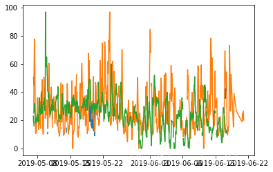
no2.pivot(columns='location',values='value').plot()
<matplotlib.axes._subplots.AxesSubplot at 0x227af5abfc8>

4.透视表:
#想要 NO2 和 PM2.5 的平均浓度以表格形式在每个站中
air_quality.pivot_table(values="value",index="location",columns="parameter",aggfunc="mean")

#当需要汇总多个值时(在这种特定情况下,pivot_table()可以使用不同时间步长的值),
#从而提供如何组合这些值的汇总函数(例如均值)。
| parameter | no2 | pm25 |
|---|---|---|
| location | ||
| BETR801 | 26.950920 | 23.169492 |
| FR04014 | 29.374284 | NaN |
| London Westminster | 29.740050 | 13.443568 |
#果同时对每个变量的摘要列感兴趣,请将margin参数放入True:
air_quality.pivot_table(values="value",index="location",columns="parameter",aggfunc="mean",margins=True)
| parameter | no2 | pm25 | All |
|---|---|---|---|
| location | |||
| BETR801 | 26.950920 | 23.169492 | 24.982353 |
| FR04014 | 29.374284 | NaN | 29.374284 |
| London Westminster | 29.740050 | 13.443568 | 21.491708 |
| All | 29.430316 | 14.386849 | 24.222743 |
air_quality.groupby(["parameter","location"]).mean()
| value | ||
|---|---|---|
| parameter | location | |
| no2 | BETR801 | 26.950920 |
| FR04014 | 29.374284 | |
| London Westminster | 29.740050 | |
| pm25 | BETR801 | 23.169492 |
| London Westminster | 13.443568 |
5. Wide to long format
- pandas.melt()方法DataFrame将数据表从宽格式转换为长格式。
- 列标题成为新创建的列中的变量名称。
[外链图片转存失败,源站可能有防盗链机制,建议将图片保存下来直接上传(img-Nqf0iDni-1595753237361)(attachment:image.png)]
#再次从上一部分中创建的宽格式表开始:
no2_pivoted = no2.pivot(columns="location", values="value").reset_index()
no2_pivoted.head()
| location | date.utc | BETR801 | FR04014 | London Westminster |
|---|---|---|---|---|
| 0 | 2019-04-09 01:00:00+00:00 | 22.5 | 24.4 | NaN |
| 1 | 2019-04-09 02:00:00+00:00 | 53.5 | 27.4 | 67.0 |
| 2 | 2019-04-09 03:00:00+00:00 | 54.5 | 34.2 | 67.0 |
| 3 | 2019-04-09 04:00:00+00:00 | 34.5 | 48.5 | 41.0 |
| 4 | 2019-04-09 05:00:00+00:00 | 46.5 | 59.5 | 41.0 |
#收集所有NO2的测量值到 单列(长格式)
no_2=no2_pivoted.melt(id_vars="date.utc")
no_2.head()
| date.utc | location | value | |
|---|---|---|---|
| 0 | 2019-04-09 01:00:00+00:00 | BETR801 | 22.5 |
| 1 | 2019-04-09 02:00:00+00:00 | BETR801 | 53.5 |
| 2 | 2019-04-09 03:00:00+00:00 | BETR801 | 54.5 |
| 3 | 2019-04-09 04:00:00+00:00 | BETR801 | 34.5 |
| 4 | 2019-04-09 05:00:00+00:00 | BETR801 | 46.5 |
#所有列id_vars一起为两列:一列与列标题名称,并用这些值本身的列。
#默认情况下,后一列的名称为value。
#pandas.melt()可以更详细地定义该方法:
no_2=no2_pivoted.melt(id_vars="date.utc",
                       value_vars=["BETR801",
                                    "FR04014",
                                    "London Westminster"],
                       value_name="NO_2",
                       var_name="id_location")
no_2.head()
| date.utc | id_location | NO_2 | |
|---|---|---|---|
| 0 | 2019-04-09 01:00:00+00:00 | BETR801 | 22.5 |
| 1 | 2019-04-09 02:00:00+00:00 | BETR801 | 53.5 |
| 2 | 2019-04-09 03:00:00+00:00 | BETR801 | 54.5 |
| 3 | 2019-04-09 04:00:00+00:00 | BETR801 | 34.5 |
| 4 | 2019-04-09 05:00:00+00:00 | BETR801 | 46.5 |
结果相同,但定义更详细:
-
value_vars明确定义要融合在一起的列
-
value_name 提供值列的自定义列名,而不是默认列名 value
-
var_name为收集列标题名称的列提供自定义列名称。否则,它采用索引名称或默认值variable
- 因此,参数value_name和var_name是两个生成的列的用户定义名称。要熔化的列由id_vars和定义value_vars。
小结:
-
支持按一列或多列排序 sort_values
-
该pivot功能是纯粹的数据重组, pivot_table支持聚合
-
pivot(长到宽格式)的相反是melt(宽到长格式)