小试牛刀

刚买到《机器学习实战》这本书，爱不释手。但是里面在调试第二章的第一处代码的时候就出现了问题，所以将一些调试结果与对其理解写在下面。

一、导入数据

由于网站的数据难以下载，数据 $csv$ 文件已经被我保存下来，百度网盘链接：https://pan.baidu.com/s/18g57CsRp5_3hYEYzjK69Vw，提取码：cg1f
数据下载下来后，在桌面创建一个文件夹，将 $csv$ 文件放入其中，另外新建一个记事本，后缀改为 $.py$ 文件，打开即可进行操作。这就是数据文件的前几行。
数据结构
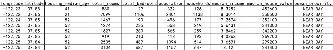
大致来看这个数据集的描述特征：longitude（纬度），latitude（经度），housing_median_age（房屋中位使用年限），total_rooms（总房间数），total_bedrooms（总卧室数），population（人口），households（家庭），median_income（平均收入），median_house_value（房屋均价），ocean_proximity（邻近海么）。翻译水平有限O_O，大致看懂了什么意思就行，一共是 $20640$ 行数据。

二、快速查看数据结构

2.1 查看数据文件形式

以下操作均在 $PythonConsole$ 下进行。

import pandas as pd
def load_housing_data(): #导入房屋数据并且返回一个pd对象
    housing_data = 'housing.csv'
    data = pd.read_csv(housing_data)
    return data
  
housing = load_housing_data()
housing.head()#调取数据前五行

   longitude  latitude  ...  median_house_value  ocean_proximity
0    -122.23     37.88  ...              452600         NEAR BAY
1    -122.22     37.86  ...              358500         NEAR BAY
2    -122.24     37.85  ...              352100         NEAR BAY
3    -122.25     37.85  ...              341300         NEAR BAY
4    -122.25     37.85  ...              342200         NEAR BAY

这里读取数据可能会出现读取不完全的情况。

longitude latitude … median_house_value ocean_proximity
0 -122.23 37.88 … 452600 NEAR BAY
1 -122.22 37.86 … 358500 NEAR BAY
2 -122.24 37.85 … 352100 NEAR BAY
3 -122.25 37.85 … 341300 NEAR BAY
4 -122.25 37.85 … 342200 NEAR BAY

在命令行里重新加入这两句就可以输出完全了。

pd.set_option('display.max_columns', None)#显示所有列
pd.set_option('display.max_rows', None)#显示所有行

2.2 查看数据空值数量

通过info()方法可以快速获取数据集的简单描述，特别是总行数，每个属性的类型和非空值的数量。

housing.info()

<class 'pandas.core.frame.DataFrame'>
RangeIndex: 20640 entries, 0 to 20639
Data columns (total 10 columns):
 #   Column              Non-Null Count  Dtype  
---  ------              --------------  -----  
 0   longitude           20640 non-null  float64
 1   latitude            20640 non-null  float64
 2   housing_median_age  20640 non-null  int64  
 3   total_rooms         20640 non-null  int64  
 4   total_bedrooms      20433 non-null  float64
 5   population          20640 non-null  int64  
 6   households          20640 non-null  int64  
 7   median_income       20640 non-null  float64
 8   median_house_value  20640 non-null  int64  
 9   ocean_proximity     20640 non-null  object 
dtypes: float64(4), int64(5), object(1)
memory usage: 1.6+ MB

我们可以看到total_bedrooms中Non-NULL Count数量为 $20433$ ，翻一翻数据文件的确存在几个空数据。

2.3 查看数据分类情况

在整个数据文件中，我们会发现除了最后一列为object属性外，其余属性均为int64，float64，那么现在我们想查看一下这个object其中到底有什么属性，后面绿色的数字是指属性出现的次数。

housing["ocean_proximity"].value_counts() #ocean_proximity为属性标签

<1H OCEAN     9136
INLAND        6551
NEAR OCEAN    2658
NEAR BAY      2290

2.4 数值属性的摘要

这里有数量，平均值，标准差，最小值，四分之一中位数等，不做过多解释了。

housing.describe()

       total_bedrooms    population    households  median_income  median_house_value  
count    20433.000000  20640.000000  20640.000000   20640.000000   20640.000000  
mean       537.870553   1425.476744    499.539680       3.870671   206855.816909  
std        421.385070   1132.462122    382.329753       1.899822   115395.615874  
min          1.000000      3.000000      1.000000       0.499900     14999.000000  
25%        296.000000    787.000000    280.000000       2.563400   119600.000000  
50%        435.000000   1166.000000    409.000000       3.534800    179700.000000  
75%        647.000000   1725.000000    605.000000       4.743250   264725.000000  
max       6445.000000  35682.000000   6082.000000      15.000100   500001.000000

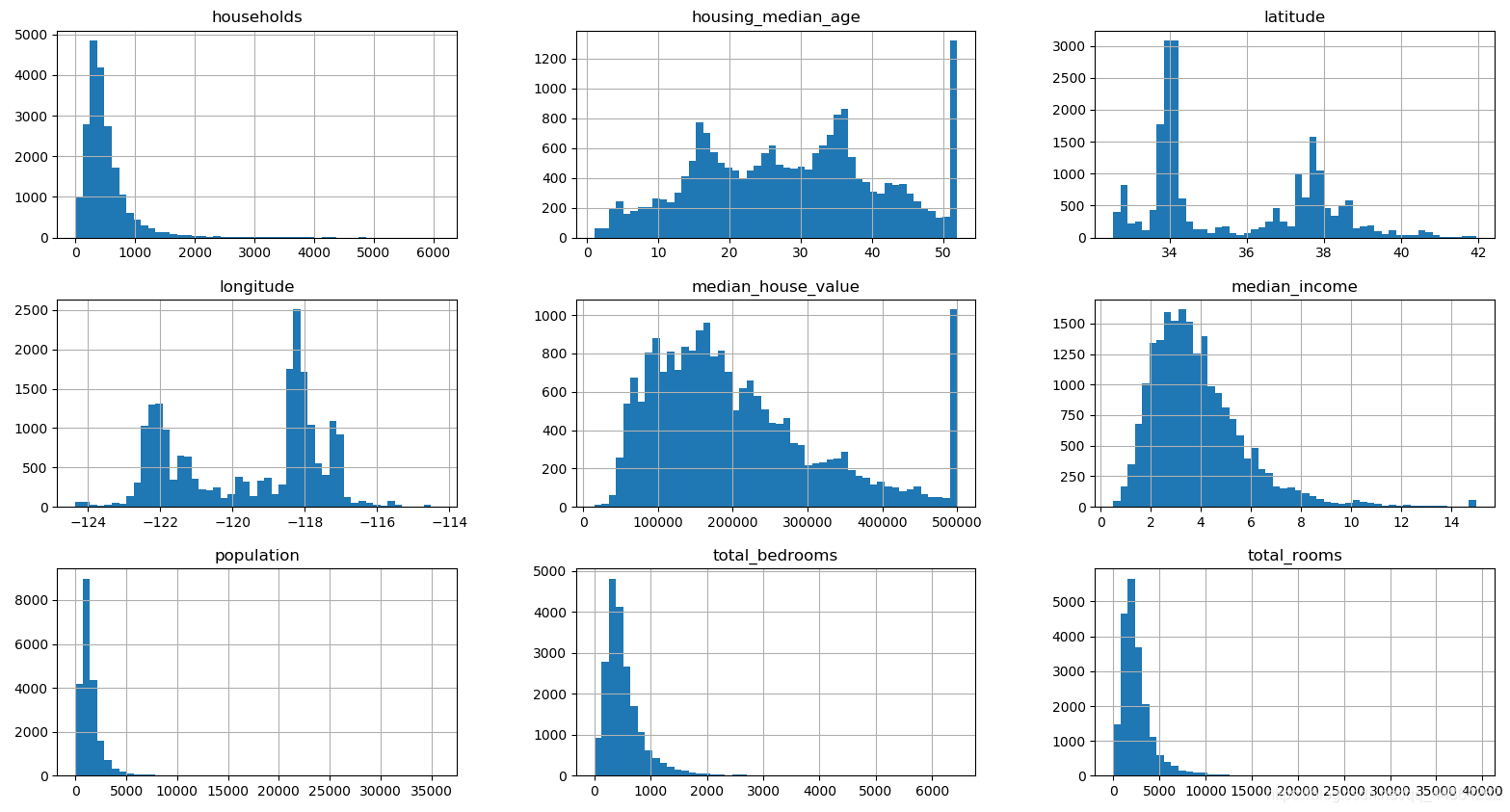
2.5 直方图展示

关于hist()函数
函数功能：在x轴上绘制定量数据的分布特征（用于连续数据，而柱状图用于离散数据）
这个可以体现数据的分布情况，画的图还不错

import matplotlib.pyplot as plt
housing.hist(bins=50,figsize=(20,15))
plt.show()

在这里插入图片描述

三、创建测试集

3.1 创建测试集

创建测试集非常简单：只需要随机选择一些实例，通常是数据集的 $20$ %，然后将他们放在一边：

import numpy as np
def split_train_test(data,test_ratio):
    shuffled_indices=np.random.permutation(len(data))#<class 'numpy.ndarray'>
    test_set_size=int(len(data)*test_ratio)#<class 'int'>
    test_indices=shuffled_indices[test_set_size]#<class 'numpy.ndarray'>
    train_indices=shuffled_indices[test_set_size:]#<class 'numpy.ndarray'>
    return data.iloc[train_indices],data.iloc[test_indices]#<class 'pandas.core.frame.DataFrame'>

train_set,test_set=split_train_test(housing,0.2)
print(len(train_set),"train + ",len(test_set),"test")

16512 train +  4128 test

np.random.permutitation()每次会产生不同的顺序集，再运行一遍又会产生不同数据集。这是创建测试集需要避免的。常见的解决方法是每个实例都是用一个标识符（identifier）来决定是否进入测试集（假定每个实例都有一个唯一且不变的标识符）。实现方式如下：

import numpy as np
import hashlib
def test_set_check(identifier,test_ratio,hash):
    return hash(np.int64(identifier)).digest()[-1]<256*test_ratio

def split_train_test_by_id(data,test_ratio,id_column,hash=hashlib.md5):
    ids = data[id_column]
    in_test_set=ids.apply(lambda id_:test_set_check(id_,test_ratio,hash))
    return data.loc[~in_test_set],data.loc[in_test_set]

housing_with_id = housing.reset_index()#使用行索引作为ID
train_set,test_set=split_train_test_by_id(housing_with_id,0.2,"index")

>>> train_set
       index  longitude  ...  median_house_value  ocean_proximity
0          0    -122.23  ...              452600         NEAR BAY
1          1    -122.22  ...              358500         NEAR BAY
2          2    -122.24  ...              352100         NEAR BAY
3          3    -122.25  ...              341300         NEAR BAY
6          6    -122.25  ...              299200         NEAR BAY
...      ...        ...  ...                 ...              ...
20634  20634    -121.56  ...              116800           INLAND
20635  20635    -121.09  ...               78100           INLAND
20636  20636    -121.21  ...               77100           INLAND
20638  20638    -121.32  ...               84700           INLAND
20639  20639    -121.24  ...               89400           INLAND

>>> test_set
       index  longitude  ...  median_house_value  ocean_proximity
4          4    -122.25  ...              342200         NEAR BAY
5          5    -122.25  ...              269700         NEAR BAY
11        11    -122.26  ...              241800         NEAR BAY
20        20    -122.27  ...              147500         NEAR BAY
23        23    -122.27  ...               99700         NEAR BAY
...      ...        ...  ...                 ...              ...
20619  20619    -121.56  ...               99100           INLAND
20625  20625    -121.52  ...               72000           INLAND
20632  20632    -121.45  ...              115600           INLAND
20633  20633    -121.53  ...               98300           INLAND
20637  20637    -121.22  ...               92300           INLAND

如果使用行索引作为唯一标识符，你需要确保在数据集的末尾添加新数据，并且不会删除任何行，如果不能保证这点，那么可以尝试使用某个最稳定的特征来创建唯一标识符。例如，一个地区的经纬度肯定几百万年都不会变，所以可以将它们组合成如下的 $ID$ ：

housing_with_id["id"] = housing["longitude"] *1000+housing["latitude"]
train_set,test_set=split_train_test_by_id(housing_with_id,0.2,"id")

>>> train_set
      index  longitude  ...  ocean_proximity         id
0          0    -122.23  ...         NEAR BAY -122192.12
1          1    -122.22  ...         NEAR BAY -122182.14
2          2    -122.24  ...         NEAR BAY -122202.15
3          3    -122.25  ...         NEAR BAY -122212.15
4          4    -122.25  ...         NEAR BAY -122212.15
...      ...        ...  ...              ...        ...
20634  20634    -121.56  ...           INLAND -121520.73
20635  20635    -121.09  ...           INLAND -121050.52
20637  20637    -121.22  ...           INLAND -121180.57
20638  20638    -121.32  ...           INLAND -121280.57
20639  20639    -121.24  ...           INLAND -121200.63

>>> test_set
       index  longitude  ...  ocean_proximity         id
8          8    -122.26  ...         NEAR BAY -122222.16
10        10    -122.26  ...         NEAR BAY -122222.15
11        11    -122.26  ...         NEAR BAY -122222.15
12        12    -122.26  ...         NEAR BAY -122222.15
13        13    -122.26  ...         NEAR BAY -122222.16
...      ...        ...  ...              ...        ...
20620  20620    -121.48  ...           INLAND -121440.95
20623  20623    -121.37  ...           INLAND -121330.97
20628  20628    -121.48  ...           INLAND -121440.90
20633  20633    -121.53  ...           INLAND -121490.81
20636  20636    -121.21  ...           INLAND -121170.51

Scikit-Learn提供了一些函数，可以通过多种方式将数据集分成多个子集。

from sklearn.model_selection import train_test_split
train_set,test_set=train_test_split(housing,test_size=0.2,random_state=42)

>>> train_set
       longitude  latitude  ...  median_house_value  ocean_proximity
14196    -117.03     32.71  ...              103000       NEAR OCEAN
8267     -118.16     33.77  ...              382100       NEAR OCEAN
17445    -120.48     34.66  ...              172600       NEAR OCEAN
14265    -117.11     32.69  ...               93400       NEAR OCEAN
2271     -119.80     36.78  ...               96500           INLAND
...          ...       ...  ...                 ...              ...
11284    -117.96     33.78  ...              229200        <1H OCEAN
11964    -117.43     34.02  ...               97800           INLAND
5390     -118.38     34.03  ...              222100        <1H OCEAN
860      -121.96     37.58  ...              283500        <1H OCEAN
15795    -122.42     37.77  ...              325000         NEAR BAY

>>> test_set
       longitude  latitude  ...  median_house_value  ocean_proximity
20046    -119.01     36.06  ...               47700           INLAND
3024     -119.46     35.14  ...               45800           INLAND
15663    -122.44     37.80  ...              500001         NEAR BAY
20484    -118.72     34.28  ...              218600        <1H OCEAN
9814     -121.93     36.62  ...              278000       NEAR OCEAN
...          ...       ...  ...                 ...              ...
15362    -117.22     33.36  ...              263300        <1H OCEAN
16623    -120.83     35.36  ...              266800       NEAR OCEAN
18086    -122.05     37.31  ...              500001        <1H OCEAN
2144     -119.76     36.77  ...               72300           INLAND
3665     -118.37     34.22  ...              151500        <1H OCEAN

3.2 测试集分层

将收入中位数除以 $1.5$ ，然后使用 $ceil$ 进行取整（得到离散类别），最后将所有大于5的类别合并为类别5

housing["income_cat"] = np.ceil(housing["median_income"]/1.5)
housing["income_cat"].where(housing["income_cat"]<5,5.0,inplace=True)

>>> housing["income_cat"]
0        5.0
1        5.0
2        5.0
3        4.0
4        3.0
        ... 
20635    2.0
20636    2.0
20637    2.0
20638    2.0
20639    2.0
Name: income_cat, Length: 20640, dtype: float64

3.3分层抽样

现在，可以根据收入类别进行分层抽样了，使用 $Scikit-Learn的Stratified-Shuffle Split$ 类：

from sklearn.model_selection import StratifiedShuffleSplit
split = StratifiedShuffleSplit(n_splits=1,test_size=0.2,random_state=42)
for train_index,test_index in split.split(housing,housing["income_cat"]):
    strat_train_set = housing.loc[train_index]
    strat_test_set = housing.loc[test_index]

可以看看所有住房数据根据收入类别的比例分布

>>> housing["income_cat"].value_counts()/len(housing)

3.0    0.350581
2.0    0.318847
4.0    0.176308
5.0    0.114438
1.0    0.039826
Name: income_cat, dtype: float64

现在可以删除Income_cat属性，将数据恢复原样了

for set in(strat_train_set,strat_test_set):
    set.drop(["income_cat"],axis=1,inplace=True)

以上就是测试集生成部分。

四、数据可视化

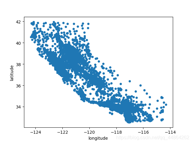
这步操作其实就是提取经纬度到x，y列表并用散点显示出来。

housing.plot(kind='scatter',x='longitude',y='latitude')

数据的地理分布图
这一步添加了一个参数 $alpha$ ，书上给出的解释是可以更清楚的看出高密度数据点的位置

housing.plot(kind='scatter',x='longitude',y='latitude',alpha=0.1)

突出该密度区域的可视化
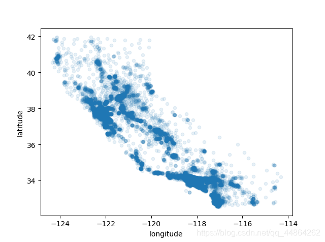
效果还不错，可以再试一试 $alpha=0.01，0.5$ 时的参数，就差不多了解这个参数是什么意思了。

housing.plot(kind='scatter',x='longitude',y='latitude',alpha=0.4,s=housing['population']/100,
			label='population',c='median_house_value',cmap=plt.get_cmap("jet"),colorbar=True)

在这里插入图片描述
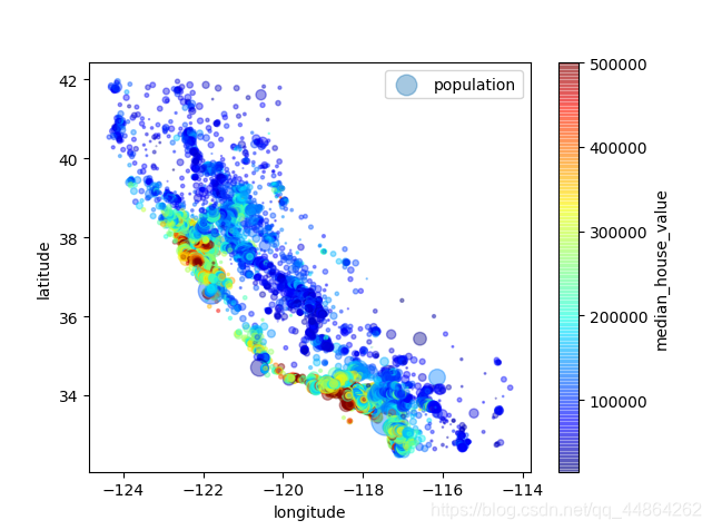
怎么可以这么漂亮，哇！

plot()参数说明

$s=housing['population']/100$ 这个就是散点的大小，没错了，人口越多的地方散点越大，很形象。
$label='population'$ ，标签，不解释也知道，看图右上角
$c$ 颜色代表价格
$cmap$ 使用一个名叫 $jet$ 的与预定义价格表，这里其实除了 $jet$ 还有挺多的， $rainbow$ ， $RdYlBu$ 都可以试一试。https://matplotlib.org/examples/color/colormaps_reference.html官方文档里面有详细的参数说明。

五、寻找相关性

可以使用corr()方法计算每对属性之间的标准相关系数（皮尔逊相关系数）

corr_matrix=housing.corr()

                    longitude  latitude  ...  median_income  median_house_value
longitude            1.000000 -0.924664  ...      -0.015176           -0.045967
latitude            -0.924664  1.000000  ...      -0.079809           -0.144160
housing_median_age  -0.108197  0.011173  ...      -0.119034            0.105623
total_rooms          0.044568 -0.036100  ...       0.198050            0.134153
total_bedrooms       0.069608 -0.066983  ...      -0.007723            0.049686
population           0.099773 -0.108785  ...       0.004834           -0.024650
households           0.055310 -0.071035  ...       0.013033            0.065843
median_income       -0.015176 -0.079809  ...       1.000000            0.688075
median_house_value  -0.045967 -0.144160  ...       0.688075            1.000000
[9 rows x 9 columns]

查看每个属性与房屋中位数的相关性分别是多少：

>>> corr_matrix["median_house_value"].sort_values(ascending=False)

median_house_value    1.000000
median_income         0.688075
total_rooms           0.134153
housing_median_age    0.105623
households            0.065843
total_bedrooms        0.049686
population           -0.024650
longitude            -0.045967
latitude             -0.144160
Name: median_house_value, dtype: float64

下面来试验一下：预测房价中位数和收入中位数的相关性散点图

housing.plot(kind='scatter',x='median_income',y='median_house_value',alpha=0.1)

在这里插入图片描述
内容来自《机器学习实战这本书》，用作学习。

《机器学习实战》加利福尼亚州房屋价格数据结构与可视化

小试牛刀

一、导入数据

二、快速查看数据结构

2.1 查看数据文件形式

2.2 查看数据空值数量

2.3 查看数据分类情况

2.4 数值属性的摘要

2.5 直方图展示

三、创建测试集

3.1 创建测试集

3.2 测试集分层

3.3分层抽样

四、数据可视化

plot()参数说明

五、寻找相关性

猜你喜欢

《机器学习实战》加利福尼亚州房屋价格 数据结构与可视化

小试牛刀

一、导入数据

二、快速查看数据结构

2.1 查看数据文件形式

2.2 查看数据空值数量

2.3 查看数据分类情况

2.4 数值属性的摘要

2.5 直方图展示

三、创建测试集

3.1 创建测试集

3.2 测试集分层

3.3分层抽样

四、数据可视化

plot()参数说明

五、寻找相关性

猜你喜欢

《机器学习实战》加利福尼亚州房屋价格数据结构与可视化