DeepDream(一)
DeepDream是什么
DeepDream能帮助我们深入了解卷积神经网络的工作原理,还能生成一些奇特、颇具艺术感的图像。
例如著名的深度学习的 “花书” 的封面就是使用DeepDream生成的。

DeepDream的原理
卷积神经网络由于其从理论上难以解释,一直被很多学者诟病。在2013年
Visualizingand Understanding Convolutional Neural Networks
这篇文章提出了使用梯度上升的方法可视化网络每一层的特征,即用一张噪声图像输入网络,反向更新的时候不更新网络权重,而是更新初始图像的像素值,以这种“训练图像”的方式可视化网络。deepdream正是以此为基础。
deepdream需要放大图像特征。比如:有一个网络学习了分类猫和狗的任务,给这个网络一张云的图像,这朵云可能比较像狗,那么机器提取的特征可能也会像狗。假设对应一个特征[0.6, 0.4],0.6表示为狗的概率, 0.4表示为猫的概率,那么采用
范数可以很好达到放大特征的效果。对于这样一个特征,
,若
越大,
越小,则
越大,所以只需要最大化
就能保证当
的时候,迭代的轮数越多
越大,
越小,所以图像就会越来越像狗。每次迭代相当于计算
范数,然后用梯度上升的方法调整图像。当然不一定要一张真实的图像,也可以从一张噪声图像生成梦境,只不过生成的梦境会比较奇怪。
以上是DeepDream的基本原理,具体实现的时候还要通过多尺度、随机移动等方法获取比较好的结果,在代码部分会给出详细解释。
实现一个简单的DeepDream
引入我们所需要的包
import tensorflow as tf
import numpy as np
import os
import time
import scipy
from PIL import Image
导入模型
在这里导入的是谷歌的 模型, 是模型的pd文件
graph = tf.Graph()
sess = tf.InteractiveSession(graph=graph)

model_fn = 'tensorflow_inception_graph.pb' # 写自己存放此文件的路径

with tf.gfile.FastGFile(model_fn,'rb') as f:
    graph_def = tf.GraphDef()
    graph_def.ParseFromString(f.read())
图像预处理
因为在训练inception模型的时候图像减了均值117.0,故在此我们也要减去此均值。
# 定义输入图像的占位符
t_input = tf.placeholder(np.float32, name='input')

# 图像预处理——减均值
imagent_mean = 117.0

# 数据预处理——增加维度
t_preprocessed = tf.expand_dims(t_input - imagent_mean,0)

# 导入模型并送入网络中
tf.import_graph_def(graph_def,{'input':t_preprocessed})
查看模型的信息
使用以下代码可以查看模型包含的所有卷积层的个数和名称
layers = [op.name for op in graph.get_operations() if op.type=='Conv2D' and 'import/' in op.name]
print('卷积层的数目为:%d' % len(layers))
print(layers)
得到的输出如下:
卷积层的数目为:59
[‘import/conv2d0_pre_relu/conv’,
‘import/conv2d1_pre_relu/conv’, ‘import/conv2d2_pre_relu/conv’,
‘import/mixed3a_1x1_pre_relu/conv’,
‘import/mixed3a_3x3_bottleneck_pre_relu/conv’,
‘import/mixed3a_3x3_pre_relu/conv’,
‘import/mixed3a_5x5_bottleneck_pre_relu/conv’,
‘import/mixed3a_5x5_pre_relu/conv’,
‘import/mixed3a_pool_reduce_pre_relu/conv’,
‘import/mixed3b_1x1_pre_relu/conv’,
‘import/mixed3b_3x3_bottleneck_pre_relu/conv’,
‘import/mixed3b_3x3_pre_relu/conv’,
‘import/mixed3b_5x5_bottleneck_pre_relu/conv’,
‘import/mixed3b_5x5_pre_relu/conv’,
‘import/mixed3b_pool_reduce_pre_relu/conv’,
‘import/mixed4a_1x1_pre_relu/conv’,
‘import/mixed4a_3x3_bottleneck_pre_relu/conv’,
‘import/mixed4a_3x3_pre_relu/conv’,
‘import/mixed4a_5x5_bottleneck_pre_relu/conv’,
‘import/mixed4a_5x5_pre_relu/conv’,
‘import/mixed4a_pool_reduce_pre_relu/conv’,
‘import/mixed4b_1x1_pre_relu/conv’,
‘import/mixed4b_3x3_bottleneck_pre_relu/conv’,
‘import/mixed4b_3x3_pre_relu/conv’,
‘import/mixed4b_5x5_bottleneck_pre_relu/conv’,
‘import/mixed4b_5x5_pre_relu/conv’,
‘import/mixed4b_pool_reduce_pre_relu/conv’,
‘import/mixed4c_1x1_pre_relu/conv’,
‘import/mixed4c_3x3_bottleneck_pre_relu/conv’,
‘import/mixed4c_3x3_pre_relu/conv’,
‘import/mixed4c_5x5_bottleneck_pre_relu/conv’,
‘import/mixed4c_5x5_pre_relu/conv’,
‘import/mixed4c_pool_reduce_pre_relu/conv’,
‘import/mixed4d_1x1_pre_relu/conv’,
‘import/mixed4d_3x3_bottleneck_pre_relu/conv’,
‘import/mixed4d_3x3_pre_relu/conv’,
‘import/mixed4d_5x5_bottleneck_pre_relu/conv’,
‘import/mixed4d_5x5_pre_relu/conv’,
‘import/mixed4d_pool_reduce_pre_relu/conv’,
‘import/mixed4e_1x1_pre_relu/conv’,
‘import/mixed4e_3x3_bottleneck_pre_relu/conv’,
‘import/mixed4e_3x3_pre_relu/conv’,
‘import/mixed4e_5x5_bottleneck_pre_relu/conv’,
‘import/mixed4e_5x5_pre_relu/conv’,
‘import/mixed4e_pool_reduce_pre_relu/conv’,
‘import/mixed5a_1x1_pre_relu/conv’,
‘import/mixed5a_3x3_bottleneck_pre_relu/conv’,
‘import/mixed5a_3x3_pre_relu/conv’,
‘import/mixed5a_5x5_bottleneck_pre_relu/conv’,
‘import/mixed5a_5x5_pre_relu/conv’,
‘import/mixed5a_pool_reduce_pre_relu/conv’,
‘import/mixed5b_1x1_pre_relu/conv’,
‘import/mixed5b_3x3_bottleneck_pre_relu/conv’,
‘import/mixed5b_3x3_pre_relu/conv’,
‘import/mixed5b_5x5_bottleneck_pre_relu/conv’,
‘import/mixed5b_5x5_pre_relu/conv’,
‘import/mixed5b_pool_reduce_pre_relu/conv’,
‘import/head0_bottleneck_pre_relu/conv’,
‘import/head1_bottleneck_pre_relu/conv’]
使用以下代码查看某一层的具体参数
# 输出某一层的参数
name = 'mixed4d_3x3_bottleneck_pre_relu'
print('Shape of %s:%s' % (name,str(graph.get_tensor_by_name('import/'+name+':0').get_shape())))
输出如下:
Shape of mixed4d_3x3_bottleneck_pre_relu:(?, ?, ?, 144)
其中144是通道数,如果选择卷积层某一个通道生成图像的话就不可以超出最大通道数。
定义保存图片函数
在此定义一个保存图片的函数
def saveimg(img_array,img_name):
    PIL.Image.fromarray(img_array).save(img_name)
    print("img saved:%s" % img_name)
定义生成函数
def render_naive(t_obj,img0,iter_n,step=0.8):

    # t_obj 为某一卷积层tf.Tensor类型的变量
    # img0 为生成的或者读取的图片
    # iter_n 为迭代轮数
    # step 为每次迭代改变的大小,类似于学习率

    t_score = tf.reduce_mean(t_obj)
    t_grad = tf.gradients(t_score,t_input)[0] # 计算输入的图像和卷积层的图像的梯度

    img = img0.copy()

    for i in range(iter_n):
        g, score = sess.run([t_grad,t_score],feed_dict={t_input:img})
        g /= g.std() + 1e-8
        img += g*step
        print("iter:%d"%(i+1),"score_mean=%f"%score)
    saveimg(img.astype( np.uint8 ), "deepdream.jpg")
生成DeepDream图片
# 选取的通道名,记得去掉 import/
name = 'mixed3b_5x5_bottleneck_pre_relu/conv'
channel = 30 # 选取的卷积层的通道数
iter_n = 100 # 迭代次数

# 获得卷积层的Tensor值
layer_output = graph.get_tensor_by_name("import/%s:0" % name)

# 随机生成噪声图片
image = np.random.uniform(size=(224,224,3))+100.0

# 使用某一特定的通道
# render_naive(layer_output[:,:,:,channel],image,iter_n=iter_n)

# 使用卷积层所有通道
render_naive(layer_output,image,iter_n=iter_n)

im = PIL.Image.open('deepdream.jpg')
im.show()
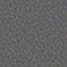
使用此较底层卷积层生成的图像如下,可见此图片还是有一定的规律的。
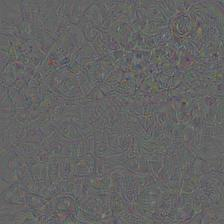
如果将通道更改为较高层的
后可见生成的图片更加抽象,不可名状。这也反映出在卷积神经网络中越底层的卷积层提取的特征越具体,越顶层的卷积层提取的特征越抽象。
后记
因为篇幅不易过长,故将更复杂的图像处理放到下一篇博客中,按照下一篇博客可实现如下效果:
原图:

DeepDream-one:

DeepDream-two:
