小白带你用Numpy、Tensor、Autograd、TensorFlow等技术实现同一个机器学习任务

1.标量方向传播

1.1 代码

import torch
#定义输入张量x
x=torch.Tensor([3])
print(x)
#初始化权重参数W,偏移量b、并设置require_grad属性为True，为自动求导
w=torch.randn(1,requires_grad=True)
b=torch.randn(1,requires_grad=True)

print("w=",w)
print("b=",b)

#实现前向传播
y=torch.mul(w,x)  #等价于w*x
print(y)
z=torch.add(y,b)
print(z)#等价于y+b
#查看x,w，b页子节点的requite_grad属性
print("x,w,b的require_grad属性分别为：{},{},{}".format(x.requires_grad,w.requires_grad,b.requires_grad))

w、x、b都是标量

tensor([3.])
w= tensor([-0.7623], requires_grad=True)
b= tensor([-0.3039], requires_grad=True)
tensor([-2.2870], grad_fn=<MulBackward0>)
tensor([-2.5909], grad_fn=<AddBackward0>)
x,w,b的require_grad属性分别为：False,True,True

1.2 查看其它属性

import torch
#定义输入张量x
x=torch.Tensor([3])

#初始化权重参数W,偏移量b、并设置require_grad属性为True，为自动求导
w=torch.randn(1,requires_grad=True)
b=torch.randn(1,requires_grad=True)

#实现前向传播
y=torch.mul(w,x)  #等价于w*x

z=torch.add(y,b)

#查看x,w，b页子节点的requite_grad属性
print("各点require_grad属性\nx.require_grad={}\nw.require_grad={}\nb.require_grad={}".format(x.requires_grad,w.requires_grad,b.requires_grad))
print("y.require_grad={}\nz.require_grad={}\n".format(y.requires_grad,z.requires_grad))
#因与w，b有依赖关系，故y，z的requires_grad属性也是：True,True
#查看各节点是否为叶子节点
print("各点是否是叶子节点\nx.is_leaf={}\nw.is_leaf={}\nb.is_leaf={}\ny.is_leaf={}\nz.is_leaf={}\n".format(x.is_leaf,w.is_leaf,b.is_leaf,y.is_leaf,z.is_leaf))
#x，w，b，y，z的是否为叶子节点：True,True,True,False,False
#查看叶子节点的grad_fn属性
print("各点grad_fn属性\nx.grad_fn={}\nw.grad_fn={}\nb.grad_fn={}\n".format(x.grad_fn,w.grad_fn,b.grad_fn))
#因x，w，b为用户创建的，为通过其他张量计算得到，故x，w，b的grad_fn属性：None,None,None
#查看非叶子节点的grad_fn属性
print("非叶子节点的grad_fn属性\ny.grad_fn={}\nz.grad_fn={}".format(y.grad_fn,z.grad_fn))

1.2.1 运行结果

各点require_grad属性
x.require_grad=False
w.require_grad=True
b.require_grad=True
y.require_grad=True
z.require_grad=True

各点是否是叶子节点
x.is_leaf=True
w.is_leaf=True
b.is_leaf=True
y.is_leaf=False
z.is_leaf=False

各点grad_fn属性
x.grad_fn=None
w.grad_fn=None
b.grad_fn=None

非叶子节点的grad_fn属性
y.grad_fn=<MulBackward0 object at 0x108d41fd0>
z.grad_fn=<AddBackward0 object at 0x108d43050>

1.2.2 自动求导

参数w,b,x的梯度分别为:tensor([3.]),tensor([1.]),None
非叶子节点y,z的梯度分别为:None,None

2.定义叶子节点和计算节点

y.backward(torch.Tensor([[1, 0]]),retain_graph=True)

J[0]=x.grad
#梯度累加的，故需要对x的梯度清零
x.grad = torch.zeros_like(x.grad)
#生成y2对x的梯度
y.backward(torch.Tensor([[0, 1]]))
J[1]=x.grad
#显示jacobian矩阵的值
print(J)

2.1运行结果

tensor([[4., 3.],[2., 6.]])

3.numpy  构建一个机器学习模型

y=wx**2+b的2个参数 w,b

3.1 代码

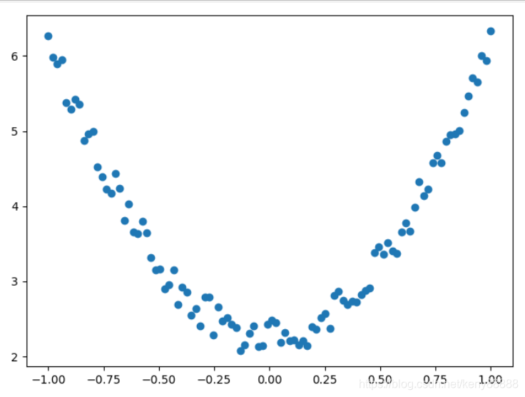
y=4X**2+2+0.5*一个随机数

import matplotlib
import numpy as np
#%matplotlib inline
from matplotlib import pyplot as plt
np.random.seed(100)
x = np.linspace(-1, 1, 100).reshape(100,1)
y = 4*np.power(x, 2) +2+ 0.5*np.random.rand(x.size).reshape(100,1)
#y=4X**2 +2+ 一个随机数
plt.scatter(x, y)
plt.show()

3.2运行效果

3.3 稍微变一下

y = 4*np.power(x, 2) +2+ 0.1*np.random.rand(x.size).reshape(100,1)

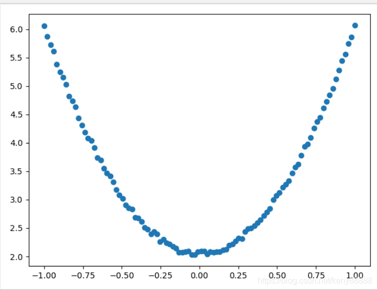
3.4 再变一下

y = 4*np.power(x, 2) +2+ 0.01*np.random.rand(x.size).reshape(100,1)

3.5 初始化权重和训练模型

w1=np.random.rand(1,1)
b1=np.random.rand(1,1)

#loss
lr=0.001
for i in range(800):
    y_pred = np.power(x,2)*w1+b1
    loss= 0.5*(y_pred - y )**2
    loss= loss.sum()
    grad_w = np.sum((y_pred- y)*np.power(x,2))
    grad_b = np.sum((y_pred -y))
    w1 -= lr*grad_w
    b1 -= lr*grad_b
#show
plt.plot(x, y_pred,'r-',label='predict')
plt.scatter(x, y,color='b',marker='o',label='true') # true data
plt.xlim(-1,1)
plt.ylim(2,6)
plt.legend()
plt.show()
print(w1,b1)

3.6 Numpy可视化学习结果

Numpy可视化学习结果

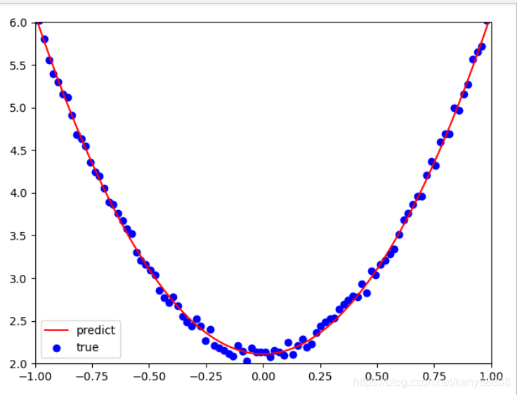
学习效果  [[3.97847587]] [[2.11193361]] 从结果看，学习效果还是比较理想的。

4.通过Tensor和autograd 自动梯度进行学习

4.1 源代码

import matplotlib
import numpy as np
import torch as t
from matplotlib import pyplot as plt

#%matplotlib inline
t.manual_seed(100) #生成训练数据
dtype=t.float #定义为float类型

x=t.unsqueeze(t.linspace(-1,1,100),dim=1)

y = 4*x.pow(2) +2+ 0.2*t.rand(x.size())
# #y=4X**2 +2+ 一个随机数
plt.scatter(x.numpy(), y.numpy())
plt.show()

ires_grad=True
w=t.rand(1,1,dtype=dtype,requires_grad=True)
b=t.zeros(1,1,dtype=dtype,requires_grad=True)


#loss
lr=0.001
for i in range(800):
    y_pred = x.pow(2)*w+b
    loss= 0.5*(y_pred - y )**2
    loss= loss.sum()
    loss.backward()
    with t.no_grad():
        w -= lr * w.grad
        b -= lr * b.grad
        w.grad.zero_()
        b.grad.zero_()

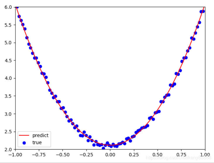
#show
plt.plot(x.numpy(), y_pred.detach().numpy(),'r-',label='predict')#predict
plt.scatter(x.numpy(), y.numpy(),color='blue',marker='o',label='true') # true data
plt.xlim(-1,1)
plt.ylim(2,6)
plt.legend()
plt.show()
print(w, b)

4.2 运行结果

学习效果

tensor([[3.9637]], requires_grad=True) tensor([[2.1149]], requires_grad=True)从结果看，学习效果和numpy差不多，还是比较理想的。

5.通过TensorFlow框架来学习训练

 5.1 源代码

# -*- coding: utf-8 -*-
#import tensorflow as tf
import tensorflow.compat.v1 as tf  #替换到tf1上的函数，tf.placeholder这个在tf1上执行
tf.disable_v2_behavior()
import numpy as np
from matplotlib import pyplot as plt
#生成训练数据
np.random.seed(100)
x = np.linspace(-1, 1, 100).reshape(100,1)
y = 4*np.power(x, 2) +2+ 0.2*np.random.rand(x.size).reshape(100,1)
#创建两个占位符，分别用来存放输入数据x和目标值y
# 运行计算图时，导入数据.

x1 = tf.placeholder(tf.float32, shape=(None, 1))
y1 = tf.placeholder(tf.float32, shape=(None, 1))
# 创建权重变量w和b，并用随机值初始化.
# TensorFlow 的变量在整个计算图保存其值.
w = tf.Variable(tf.random_uniform([1], 0, 1.0))
b = tf.Variable(tf.zeros([1]))
# 前向传播，计算预测值.
y_pred = np.power(x,2)*w + b
# 计算损失值
loss=tf.reduce_mean(tf.square(y-y_pred))
# 计算有关参数w、b关于损失函数的梯度.
grad_w, grad_b = tf.gradients(loss, [w, b])
#用梯度下降法更新参数.
# 执行计算图时给 new_w1 和new_w2 赋值
# 对TensorFlow 来说，更新参数是计算图的一部分内容
# 而PyTorch，这部分属于计算图之外.
learning_rate = 0.01
new_w = w.assign(w - learning_rate * grad_w)
new_b = b.assign(b - learning_rate * grad_b)

# 已构建计算图，接下来创建TensorFlow session，准备执行计算图.
with tf.Session() as sess:
    # 执行之前需要初始化变量w、b
    sess.run(tf.global_variables_initializer())
    for step in range(2000):
        # 循环执行计算图. 每次需要把x1、y1赋给x和y.
        # 每次执行计算图时，需要计算关于new_w和new_b的损失值,
        # 返回numpy多维数组
        loss_value, v_w, v_b = sess.run([loss, new_w, new_b],
                                    feed_dict={x1: x, y1: y})
        if  step%200==0:  #每200次打印一次训练结果
            print("损失值、权重、偏移量分别为{:.4f},{},{}".format(loss_value,v_w,v_b))
#
# 可视化结果
plt.figure()
plt.scatter(x,y)
plt.plot (x, v_b + v_w*x**2)

5.2 运行结果

5.3 运行效果

损失值、权重、偏移量分别为11.1054,[0.8165218],[0.0637291]
损失值、权重、偏移量分别为0.2246,[2.4479122],[2.6355228]
损失值、权重、偏移量分别为0.1174,[2.8882298],[2.5057666]
损失值、权重、偏移量分别为0.0624,[3.1974423],[2.3915539]
损失值、权重、偏移量分别为0.0339,[3.4199224],[2.3091285]
损失值、权重、偏移量分别为0.0192,[3.5800555],[2.2497995]
损失值、权重、偏移量分别为0.0116,[3.6953108],[2.2070973]
损失值、权重、偏移量分别为0.0076,[3.778269],[2.176361]
损失值、权重、偏移量分别为0.0055,[3.8379784],[2.1542387]
损失值、权重、偏移量分别为0.0045,[3.8809562],[2.1383154]

5.4 训练数调整

损失值、权重、偏移量分别为11.5526,[0.6570691],[0.06481812]
...
损失值、权重、偏移量分别为0.0034,[3.979565],[2.1017814]
损失值、权重、偏移量分别为0.0033,[3.9828653],[2.1005585]

损失值、权重、偏移量分别为0.0033,[3.9828653],[2.1005585]这个值是最好的值

损失值越小越好, 权重接近4，偏移量接近2 。

6.总结

熟悉分别用Numpy、Tensor、Autograd、TensorFlow等技术实现同一个机器学习任务。