本文主要记录:
1. 离散特征如何预处理之后嵌入
2.使用pytorch怎么使用nn.embedding
以推荐系统中:考虑输入样本只有两个特征,用逻辑回归来预测点击率ctr
看图混个眼熟,后面再说明:
一、离散数据预处理
假设一个样本有两个离散特征【职业,省份】,第一个特征种类有10种,第二个特征种类有20种。于是field_dims=[10, 20]
“职业”的取值为:[学生,老师,老板,司机……]共10种
“省份”的取值为:[黑龙江、吉林、四川(第3个位置)、……、北京(第7个位置)、……、重庆(第19个位置)、……]
设原始数据部分样本是这样的(标签没写出来,点击就为1,未点击就为0):
[学生,四川],[学生,北京],[老师,重庆]
那么处理过后变为
[1, 3], [1, 7], [2, 19]
假设我们在torch嵌入方式为:所有特征同时一起嵌入(还有就是分别嵌入:就是每个特征分开嵌入,然后把所有特征的嵌入向量用torch.cat拼接成一个向量):
field_dims=[10,20],取embed_dim=3
Self.embed = torch.nn.Embedding(sum(field_dims), embed_dim)
这个时候得到了一个索引字典index_dict,长度为sum(field_dims)=30, 每个索引对应一个嵌入维度为embed_dim=3的向量(相当于字典的key为1到30,每个key对应一个嵌入的维度为embed_dim=3的向量)
现在,我们该怎么把[学生,四川],对应的[1, 3]数据嵌入进去,嵌入的结果是什么呢?
这个时候需要把[1, 3], [1, 7], [2, 19]变为[1, 13], [1, 17], [2, 29].
因为在one-hot编码的时候[1, 3]中的1对应“1,0,0,0,0,0,0,0,0,0”,3对应“0,0,1,0,0,0,0,0,0,0,0,0,0,0,0,0,0,0,0,0”,
最终形成的one-hot向量为“1,0,0,0,0,0,0,0,0,0,0,0,1,0,0,0,0,0,0,0,0,0,0,0,0,0,0,0,0,0”,1和3分别在第1位置和第13位置(我把这种操作简单叫做:变换处理)。
设batch_size=2,那么在定义模型的时候,def forward(self, x)中的x的size就等于batch_size*特征数=2*2。
假如第一个batch读取的数据是[1, 3], [1, 7], 则x=[[1,3], [1,7]],经过“变换处理”变为了x_=[[1,13], [1,17]],
这个时候就可以把x_输入到嵌入层,embed_result = Self.embed(x_)
得到的结果embed_result的size为:batch_size*特征数*嵌入维度=2*2*3。
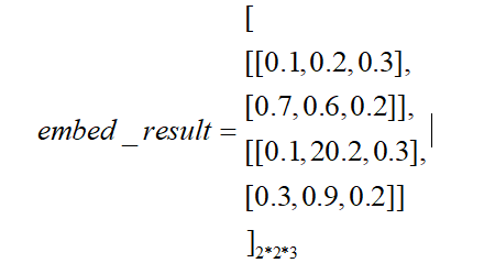
设1,13,17对应的嵌入向量分为为[0.1, 0.2, 0.3], [0.3, 0.6, 0.2], [0.3, 0.9, 0.2],
那么embed_result结果为(还是一个tensor,这儿只是展现了数据):
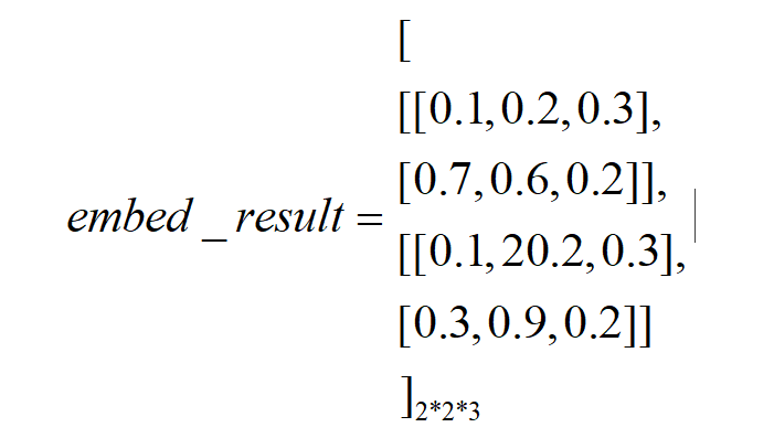
因为batch_size=2,是两个样本,所以最后需要得到两个输出。
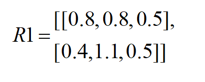
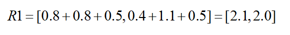
R1 = torch.sum(embed_result,1) # size=batch_size*嵌入维度=2*3
[0.1+0.7, 0.2+0.6, 0.3+0.2] = [0.8, 0.8, 0.5]
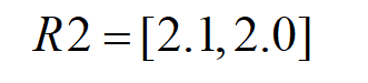
R2 = torch.sum(R1,1) # size = batch_size=2
(注意,如果还要在添加层的话,可以把R1作为下一层的输入,或者把embed_result每一个样本的特征拼接起来得到R3输入到下一层)
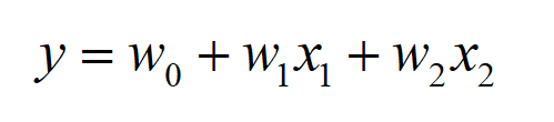
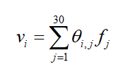
上面这个怎么和公式![]() 联系起来呢,感觉直接是把特征嵌入过后的向量直接相加求和得到输出y,公式前面的权重w怎么体现的呢?
联系起来呢,感觉直接是把特征嵌入过后的向量直接相加求和得到输出y,公式前面的权重w怎么体现的呢?
因为特征x1有10个取值,x2有20个取值,one-hot编码过后,特征变成了30个,设新的特征为f:

原来的式子![]() 相当于变成了:
相当于变成了:

对于样本[学生,四川]—>[1,3]-变换处理->[1, 13],
![]() 只有x1,1一个为1,
只有x1,1一个为1,
![]() 其中也只有x2,3一个为1
其中也只有x2,3一个为1
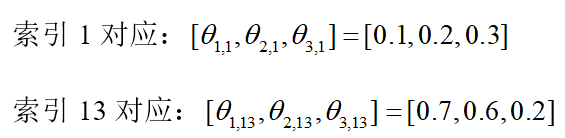
然而实际上并没有采用one-hot存储,当用了embedding过后只是存储了一个索引字典,设嵌入的为度为3,式子相当于(设θ0=0)

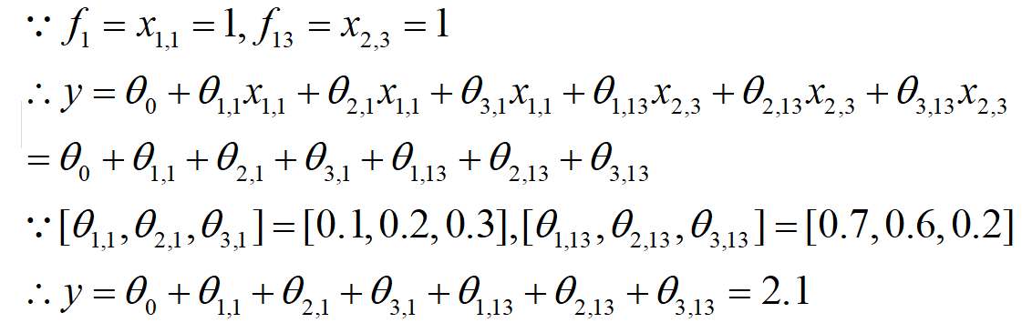
这就与R2中的结果对应上了。所以直接把样本嵌入向量的元素值全部加起来,就是输出。
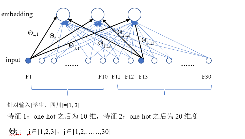
图解:
针对输入为[学生,四川]-->[1,3]-->[1, 13],
输入层one-hot编码第1个位置和第13个位置是1(蓝色),其余位置是0
(启示程序中并不是输入的one-hot编码,只是一个索引key=1和13,通过索引去得到嵌入过后的向量)

1.嵌入
embed_result = Self.embed(x_)
2.每个特征的对应元素求和,得到embedding层第i个神经元的值
对应代码R1 = torch.sum(embed_result,1)。# size=batch_size*嵌入维度=2*3
比如,以输入[1,3]à[1,13]为例,

得到嵌入层三个神经元的值为:
![]()
同理计算得到[1,7]-->[1,17]对应的embedding层神经元的值
![]()
即: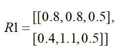
3. 把每个样本embeding层所有神经元的值加起来。
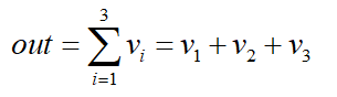
对应代码R2 = torch.sum(R1, 1) # size = batch_size=2
补充说明
特征嵌入的两种方式
1.所有特征一起嵌入
field_dims=[10,20], emb_dim1=3, 设batch_size=2x1=[1, 3],x2=[1,7],
于是一个batch中 x=[[1, 3], [1, 7]],
Pytorch代码:
embed_1 = torch.nn.Embedding(sum(field_dims), emb_dim1)
x “变换处理”后,得到x_=[[1, 13], [1, 17]]
输入x_,输出embed_result1
embed_result1 = embed_1(x_)#size=batch_size*特征数*嵌入维度=2*2*3
此时需要用r1 = torch.sum(embed_result1, 1)得到的结果size=2*3
r2 = torch.sum(r1,1) # size = batch_size =2
ebd = nn.Embedding(30,3)
x_ =  Variable(torch.LongTensor([[1, 13], [1, 17]]))
print(ebd(x_))  #2*2*3
r1 = torch.sum(ebd(x_),1)
print(r1)  # 2*3
r2 = torch.sum(r1,1)
print(r2) #size = 2
输出;
tensor([[[ 2.2919,  0.2820, -0.0129],
         [-0.1115,  2.2074,  0.1836]],

        [[ 2.2919,  0.2820, -0.0129],
         [ 1.0564,  0.4073, -1.7239]]], grad_fn=<EmbeddingBackward>)
tensor([[ 2.1804,  2.4893,  0.1707],
        [ 3.3483,  0.6892, -1.7368]], grad_fn=<SumBackward1>)
tensor([4.8404, 2.3007], grad_fn=<SumBackward1>)
2.特征分别嵌入,然后再cat。
(比如,模型准备把嵌入维度设为100,同时嵌入的嵌入维度直接为100,分别嵌入各个特征的嵌入维度之和为100)
(同时嵌入的嵌入维度为3,为了保持一致,分别嵌入时候第一个特征嵌入维度设为1,第二个特征设嵌入维度为2)
field_dims=[10,20], emb_dim2_1=1, emb_dim2_1=2
embed2_1 = torch.nn.Embedding(filed_dims[0], emb_dim2_1)
embed2_2 = torch.nn.Embedding(filed_dims[1], emb_dim2_2)
embed_result2_1 = embed2_1(x_[ : ,0]) #batch_size*emb_dim2_1=2*1
#相当于得到对[1, 1]嵌入的结果
embed_result2_2 = embed2_2(x_[ : ,1]) #batch_size*emb_dim2_1=2*2
#相当于得到对[13, 17]嵌入的结果
embed_result_list = embed_result2_1+ embed_result2_2
embed_result2 = torch.cat(embed_result_list, 1) #size=batch_size*( emb_dim2_1+ emb_dim2_2=2*1*(1+2)=2*3
最后使用torch.sum(embed_result2, 1) # size=2
x_ =  Variable(torch.LongTensor([[1, 13], [1, 17]]))
embed2_1 = nn.Embedding(10,1)
embed2_2 = nn.Embedding(20,2)
embed_result2_1 = embed2_1(x_[ : ,0])
embed_result2_2 = embed2_2(x_[ : ,1])
print(embed_result2_1)  # batch_size*emb_dim2_1=2*1
print(embed_result2_2)  #batch_size*emb_dim2_1=2*2
lisi_ebd2 = []
lisi_ebd2.append(embed_result2_1)
lisi_ebd2.append(embed_result2_2)
# lisi_ebd2长度为2,一个元素为2*1大小,一个元素为2*2
embed_result2 = torch.cat(lisi_ebd2,1)
print(embed_result2)  #2*3
p = torch.sum(embed_result2, 1)
print(p)  # size=2

输出:
tensor([[0.4481],
        [0.4481]], grad_fn=<EmbeddingBackward>)
tensor([[ 0.7232,  0.6618],
        [-1.4629,  1.1546]], grad_fn=<EmbeddingBackward>)
tensor([[ 0.4481,  0.7232,  0.6618],
        [ 0.4481, -1.4629,  1.1546]], grad_fn=<CatBackward>)
tensor([1.8331, 0.1397], grad_fn=<SumBackward1>)