【梯度下降算法】{1} ——模拟实现梯度下降法

此处我们模拟一下梯度下降法的实现。

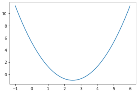
一、画出损失函数的图像：

import numpy as np
import matplotlib.pyplot as plt

plot_x = np.linspace(-1, 6, 141) # 返回-1到6均匀间隔的数字
plot_y = (plot_x-2.5)**2-1

plt.plot(plot_x, plot_y)
plt.show()

---

二、简单实现梯度下降法：

def dJ(theta):
	"""计算theta点在曲线上的导数值"""
    return 2*(theta-2.5)

def J(theta):
	"""计算theta点的损失函数值"""
    return (theta-2.5)**2-1

eta = 0.1
epsilon = 1e-8
theta = 0.0 # 初始点

while True:
    gradient = dJ(theta)
    last_theta = theta
    theta = theta - eta * gradient # 向导数的负方向移动
    
    # 判断新的theta是否来到最小值点
    if(abs(J(theta) - J(last_theta)) < epsilon):
        break
        
print(theta)
print(J(theta))

由此可以验证梯度下降法是成功的。

---

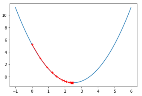
三、记录theta的变化：

theta = 0.0
theta_history = [theta]

while True:
    gradient = dJ(theta)
    last_theta = theta
    theta = theta - eta * gradient
    theta_history.append(theta)
    
    if(abs(J(theta) - J(last_theta)) < epsilon):
        break
        
plt.plot(plot_x, J(plot_x))
plt.plot(np.array(theta_history), J(np.array(theta_history)), color='r', Marker='+')
plt.show()

print("迭代次数为:" + str(len(theta_history)))

Output：

---

四、改变η（学习率）的值：

def gradient_descent(initial_theta, eta, epsilon=1e-8):
    theta = initial_theta
    theta_history.append(initial_theta)
    
    while True:
        gradient = dJ(theta)
        last_theta = theta
        theta = theta - eta * gradient
        theta_history.append(theta)
        
        if(abs(J(theta) - J(last_theta)) < epsilon):
            break
        
def plot_theta_history():
    plt.plot(plot_x, J(plot_x))
    plt.plot(np.array(theta_history), J(np.array(theta_history)), color='r', Marker='+')
    plt.show()
    
eta = 0.01
theta_history = []
gradient_descent(0, eta)
plot_theta_history()

print("迭代次数为:" + str(len(theta_history)))

Output：

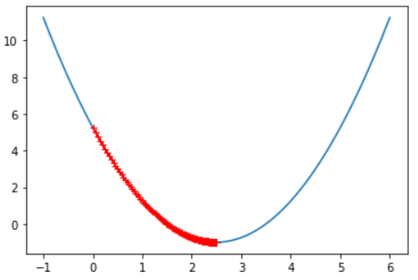
由此可知，如果η（学习率）取值太小，那么梯度下降法的速率也会减慢。

---

那如果η（学习率）的值取太大了呢？

eta = 0.8
theta_history = []
gradient_descent(0, eta)
plot_theta_history()

Output：

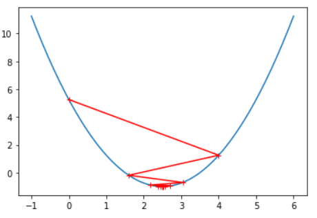
由此可知，η（学习率）取值太大，会导致梯度下降法无法收敛。

eta = 1.1
theta_history = []
gradient_descent(0, eta)

Output：

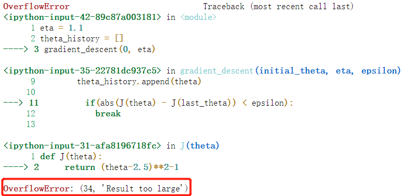
甚至溢出。

---

综上所述，eta设置小一点比较保险。

---

参考资料：bobo老师机器学习教程