tensorflow学习（6）- Mnist手写数字识别

前言

上一篇博客：tensorflow学习（5）- 用神经网络训练回归问题
这一章学习下使用Mnist数据集训练识别手写数字，并优化神经网络。

准备工作

导入包

import tensorflow as tf
from tensorflow.examples.tutorials.mnist import input_data

导入mnist数据集

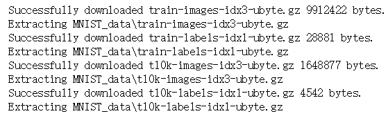
mnist = input_data.read_data_sets("MNIST_data",one_hot = True)

这会自动从网站上下载mnist数据集，这里写的下载地址是当前目录下。

给样本分批次

#每个批次的大小
batch_size = 100
#计算一共多少批次
n_batch = mnist.train.num_examples // batch_size

Tips：

• //这是整除

创建神经网络

#定义两个palceholder
x = tf.placeholder(tf.float32,[None,784])
y = tf.placeholder(tf.float32,[None,10])

#创建简单的神经网络
W = tf.Variable(tf.zeros([784,10]))
b = tf.Variable(tf.zeros([10]))
prediction = tf.nn.softmax(tf.matmul(x,W) + b)

#定义二次代价函数
loss = tf.reduce_mean(tf.square(y - prediction))
#使用梯度下降
train_step = tf.train.GradientDescentOptimizer(0.2).minimize(loss)

Tips:

• x = tf.placeholder(tf.float32,[None,784]),这里的784是28 * 28，mnist数据集中的图片大小是28*28的，因为图片是二位矩阵，这里将二维做了一个降维度的处理，把每一行都堆叠在第一行的后面这样就把28 * 28转换成了1 * 784。
• y = tf.placeholder(tf.float32,[None,10])，这里的10是十个阿拉伯数字0-9，因为识别的结果在这是个数中，如果数是5那么输出结果是[0,0,0,0,1,0,0,0,0,0]。
• prediction = tf.nn.softmax(tf.matmul(x,W) + b)，softmax他把一些输入映射为0-1之间的实数，并且归一化保证和为1，因此多分类的概率之和也刚好为1。

准备训练

#初始化变量
init = tf.global_variables_initializer()

#存放在一个bool型列表中
correct_predicition = tf.equal(tf.argmax(y,1),tf.arg_max(prediction,1))

#求准确率
accuracy = tf.reduce_mean(tf.cast(correct_predicition,tf.float32))

with tf.Session() as sess:
    sess.run(init)
    for epoch in range(200):
        for batch in range(n_batch):
            batch_xs,batch_ys = mnist.train.next_batch(batch_size)
            sess.run(train_step,feed_dict={x:batch_xs,y:batch_ys})
            
        acc = sess.run(accuracy,feed_dict={x:mnist.test.images,y:mnist.test.labels})
        print("Iter" + str(epoch) + ",Accuracy" + str(acc))

训练结果

优化方法

• 修改批次的大小
• 增加隐藏层
• 修改隐藏层的神经元数
• 修改权重偏置的初始值
• 修改代价函数
• 修改梯度下降法的学习率
• 修改别的优化方法
• 修改训练次数

4.1修改训练次数

4.1.1次数修改为100次

    for epoch in range(100):

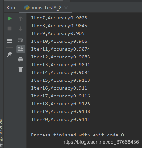
4.1.2测试结果

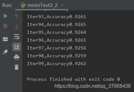
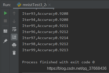
4.1.3最终结果

可以看到最终收敛在0.925左右

4.1.4总结

训练次数越多，准确率越高

4.2修改批次大小

4.2.1修改批次50

# 每个批次的大小
batch_size = 50

4.2.2测试结果

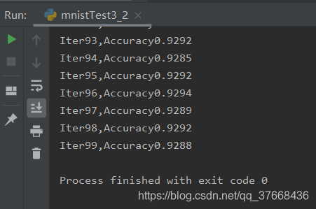
4.2.3最终结果

我们和训练一百次每个批次100对比的话发现准确率收敛在0.929左右，基本上没有变化

4.2.4修改批次200

# 每个批次的大小
batch_size = 200

4.2.5测试结果

4.2.6最终结果

训练收敛在0.921左右，没有之前效果好。

4.2.7总结

批次数越小，准确度稍微提高，效果不明显。

4.3增加隐藏层

4.3.1增加十个神经元的隐藏层

import tensorflow as tf
from tensorflow.examples.tutorials.mnist import input_data

# 载入数据
mnist = input_data.read_data_sets("MNIST_DATA", one_hot=True)

# 每个批次的大小
batch_size = 100
# 计算一共多少批次
n_batch = mnist.train.num_examples // batch_size

# 定义两个palceholder
x = tf.placeholder(tf.float32, [None, 784])
y = tf.placeholder(tf.float32, [None, 10])

#定义神经网络中间层
Weights_L1 = tf.Variable(tf.random_normal([784, 10]))
biases_L1 = tf.Variable(tf.zeros([10, ]))
Wx_plus_b_L1 = tf.matmul(x, Weights_L1) + biases_L1
#激活函数
L1 = tf.nn.sigmoid(Wx_plus_b_L1)

# 创建简单的神经网络
W = tf.Variable(tf.zeros([10, 10]))
b = tf.Variable(tf.zeros([10]))
Wx_plus_b_L2 = tf.matmul(L1, W) + b
prediction = tf.nn.softmax(Wx_plus_b_L2)

# 定义二次代价函数
loss = tf.reduce_mean(tf.square(y - prediction))
# 使用梯度下降
train_step = tf.train.GradientDescentOptimizer(0.2).minimize(loss)

# 初始化变量
init = tf.global_variables_initializer()

# 存放在一个bool型列表中
correct_predicition = tf.equal(tf.argmax(y, 1), tf.argmax(prediction, 1))

# 求准确率
accuracy = tf.reduce_mean(tf.cast(correct_predicition, tf.float32))

with tf.Session() as sess:
    sess.run(init)
    for epoch in range(1000):
        for batch in range(n_batch):
            batch_xs, batch_ys = mnist.train.next_batch(batch_size)
            sess.run(train_step, feed_dict={x: batch_xs, y: batch_ys})

        acc = sess.run(accuracy, feed_dict={x: mnist.test.images, y: mnist.test.labels})
        print("Iter" + str(epoch) + ",Accuracy" + str(acc))

4.3.2测试结果

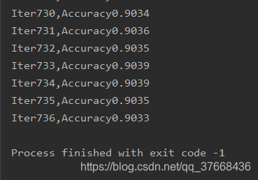
4.3.3最终结果

数据稳定在0.9左右，准确率降低了不少

4.3.4增加一百个神经元

#定义神经网络中间层
Weights_L1 = tf.Variable(tf.random_normal([784, 100]))
biases_L1 = tf.Variable(tf.zeros([100, ]))
Wx_plus_b_L1 = tf.matmul(x, Weights_L1) + biases_L1
#激活函数
L1 = tf.nn.sigmoid(Wx_plus_b_L1)

# 创建简单的神经网络
W = tf.Variable(tf.zeros([100, 10]))
b = tf.Variable(tf.zeros([10]))

4.3.5最终结果

…不贴了还是0.9出头。
但是我训练了1000次到了0.94，之前总看有过拟合的问题，是不是训练次数过多的原因啊？？？待学习学习…

4.4使用交叉熵函数

4.4.1修改loss

loss = tf.reduce_mean(tf.nn.softmax_cross_entropy_with_logits_v2(labels=y, logits=prediction))

4.4.2测试结果

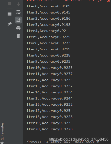
4.4.3最终结果

可以看到，收敛速度明显加快了，但是准确率还是基本不变，因为交叉熵函数是根据当前预测值与实际值的差来决定参数更新速度的，差越大更新越快，反之越小。