一、什么是模型预测控制(MPC)
MPC主要用于车道线的追踪,保持车辆轨迹相对平稳。
MPC将车道追踪任务重构成一个寻找最优解的问题,优化问题的最优解就是最优的轨迹。我们每走一步都会按照目前的状态求解一个最优化的轨迹,然后按照轨迹走一步,紧接着继续按照传感器获得的新值继续求解最优轨迹,保证轨迹跟 我们要追踪的车道线的最大拟合。这个过程中,因为我们每动一步,就是一个时间片段,因为各种误差的存在,导致我们的车辆并不能完全符合预测出来的轨迹,所以每一次都得重新计算调整。
二、车辆的模型
想要对车辆进行模型预测控制,首先我们得对车辆进行建模。这里我们对车辆的动力学模型进行一个简化,当然越复杂的模型预测起来就会更加准确,但是简单的模型更加方便计算和理解。
运动学模型
运动学模型忽略了轮胎力,重力以及质量,这种模型可以说是经过了极大的的简化,所以精确度低,但是因为经过简化,所以很好计算,而且在低中速的运动中还有这相当不错的精度
动力学模型
动力学模型是尽可能的体现出实际上车辆的动态。它计算到了轮胎的摩擦力,横向和纵向的加速度,惯性,中立,空气阻力,质量以及车辆的物理形状,所以不同的车的动力学模型很可能是不一样的,而且考虑的因素越多也就相对越精确。有的复杂的动力学模型甚至会考虑到底盘悬挂如何响应。
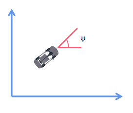
2.1 静态模型
首先我们来描述一辆车的静态的状态,那么就有坐标x,y,然后车头会有一个跟参考方向的夹角ψ。
2.2 动态模型
如果汽车动起来,那么就会增加一个参数v,即速度:
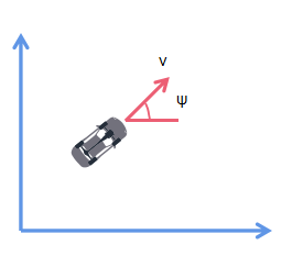
所以我们汽车的状态向量就是
X = [x,y,ψ,v]
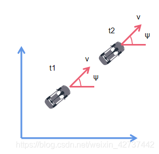
2.3 状态控制向量
我们想要控制汽车的动作,需要通过方向盘和油门踏板来实现,这里我们简化一下,把这两个都看作是单独的执行器。
δ代表方向的转动角度(注意不是方向盘的转角,而是车轮的偏向角);
a代表油门踏板的动作,正数为加速,负数为减速。
所以状态控制向量为:
[δ,a]
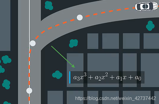
2.4 车道线的拟合
一般来说对于大多数道路,我们如果使用多项式拟合的话,那么三次多项式就足够在一定距离内比较好的拟合车道了。
2.5 各种公式
假设我们计算的时间间隔为Δt。
首先,针对位置信息x和y:

然后,对于偏向角ψ:
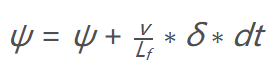
我们用到了转角加速度δ,然后Lf表示汽车的半轴长,与转弯半径相关,这个值越大,转弯半径越大。然后呢,当去读越快的时候,转弯速度也是最快的,所以速度也包含在内。
接下来就是速度:
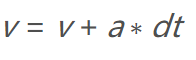
其中a为油门踏板了,取值为-1——1。
所以我们就有了一个模型:
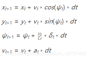
状态计算
VectorXd globalKinematic(const VectorXd &state,
                         const VectorXd &actuators, double dt) {
  // Create a new vector for the next state.
  VectorXd next_state(state.size());
  // state is [x, y, psi, v] and actuators is [delta, a]

  double x_t = state(0);
  double y_t = state(1);
  double psi_t = state(2);
  double v_t = state(3);

  double delta_t = actuators(0);
  double a_t = actuators(1);

  double x = x_t + v_t * cos(psi_t) * dt;
  double y = y_t + v_t * sin(psi_t) * dt;
  double psi = psi_t + v_t / Lf * delta_t * dt;
  double v = v_t + a_t * dt;

  next_state << x,y,psi,v;

  return next_state;
}
拟合三次曲线
#include <iostream>
#include "Eigen-3.3/Eigen/Core"
#include "Eigen-3.3/Eigen/QR"

using Eigen::VectorXd;

// Evaluate a polynomial.
double polyeval(const VectorXd &coeffs, double x);
// Fit a polynomial.
VectorXd polyfit(const VectorXd &xvals, const VectorXd &yvals, int order);

int main() {
  VectorXd xvals(6);
  VectorXd yvals(6);
  // x waypoint coordinates
  xvals << 9.261977, -2.06803, -19.6663, -36.868, -51.6263, -66.3482;
  // y waypoint coordinates
  yvals << 5.17, -2.25, -15.306, -29.46, -42.85, -57.6116;


  auto coeffs = polyfit(xvals, yvals, 3);

  for (double x = 0; x <= 20; ++x) {

    std::cout << polyeval(coeffs,x) << std::endl;
  }

}

double polyeval(const VectorXd &coeffs, double x) {
  double result = 0.0;
  for (int i = 0; i < coeffs.size(); ++i) {
    result += coeffs[i] * pow(x, i);
  }
  return result;
}

// Adapted from:
// https://github.com/JuliaMath/Polynomials.jl/blob/master/src/Polynomials.jl#L676-L716
VectorXd polyfit(const VectorXd &xvals, const VectorXd &yvals, int order) {
  assert(xvals.size() == yvals.size());
  assert(order >= 1 && order <= xvals.size() - 1);

  Eigen::MatrixXd A(xvals.size(), order + 1);

  for (int i = 0; i < xvals.size(); ++i) {
    A(i, 0) = 1.0;
  }

  for (int j = 0; j < xvals.size(); ++j) {
    for (int i = 0; i < order; ++i) {
      A(j, i + 1) = A(j, i) * xvals(j);
    }
  }

  auto Q = A.householderQr();
  auto result = Q.solve(yvals);

  return result;
}
2.6 误差计算
我们通过将误差最小化作为调优的目标。
我们新的状态向量是 [x,y,ψ,v,cte,eψ].
2.6.1 航向偏差
航向偏差表示汽车的行进路线与道路中心线的偏差,
ctet+1=ctet+vt∗sin(eψt)∗dt
ctet可以表示为车辆当前位置与yt(道路中心线)之间的差值,所以有:
ctet=f(xt)−yt
然后带入上式可得:
ctet+1=f(xt)−yt+vt∗sin(eψt)∗dt
其中的误差可以分为两部分:
- f(xt)−yt为当前的航迹偏差
- vt∗sin(eψt)∗dt为车辆运动引起的偏差
2.6.2 方向偏差
接下来就是方向偏差:
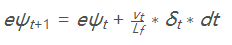
计算方法跟ψ类似。
eψt的计算方法是使用eψt减去目标角度。
eψt = ψt - ψdest
ψt是已知的,但是ψdest是未知的,我们只知道路径的多项式,我们可以使用当前点的正切角来计算这个值,arctan(f′ (xt)),f′是轨迹的导数。
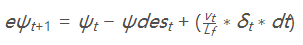
- eψt是当前的方向偏差
- 后部分是速度造成的偏差
三、MPC的实现
3.1 工具
这里我们用到两个工具,辅助我们的计算
3.1.1 Ipopt
ipopt是一个解决非线性规划最优化问题的工具集,当然,它也能够用于解决线性规划问题的求解。
ipopt可以根据我们的约束条件来求解局部最优,所以很适用与非线性问题。但是这个工具要求我们提供约束条件的Jacobian矩阵和目标函数的Hessian矩阵,这个其实还是比较费劲的,所以我们有了以下的工具:CppAD
3.1.2 CppAD
CppAD是一个自动计算导数的工具,
为了使用其计算导数,我们所有的计算函数以及数据类型都需要使用这个包里自带的。例如:
CppAD::pow(x, 2);
// instead of
pow(x, 2);
3.2 初始化
首先设置各种初始化的值
/**
 *  设置时间间隔和预测的步数
 */
size_t N = 10;
double dt = 0.1;


//设置半轴长
const double Lf = 2.67;

//设置目标车速
double ref_v = 40.0;

// 定义每一个state的起始点,因为函数的需要,只能传入一个数组,所以将误差以及各种状态的点都放在一个数组中展开
size_t x_start = 0;
size_t y_start = x_start + N;
size_t psi_start = y_start + N;
size_t v_start = psi_start + N;
size_t cte_start = v_start + N;
size_t epsi_start = cte_start + N;
size_t delta_start = epsi_start + N;
size_t a_start = delta_start + N - 1;
3.3 设置约束
class FG_eval {
 public:
  // Fitted polynomial coefficients
  VectorXd coeffs;
  FG_eval(VectorXd coeffs) { this->coeffs = coeffs; }

  typedef CPPAD_TESTVECTOR(AD<double>) ADvector;
  void operator()(ADvector& fg, const ADvector& vars) {
// The cost is stored is the first element of `fg`.
    // Any additions to the cost should be added to `fg[0]`.
    fg[0] = 0;

    // Reference State Cost

    // 损失函数,目的是将损失函数降到最小,求最优化解
    //基于参考状态的损失,求状态的最优化,最小的距离,最小的夹角,最小的速度
    for (unsigned int i = 0; i < N; i++)
    {
      fg[0] += 500 * CppAD::pow(vars[cte_start + i], 2);
      fg[0] += 500 * CppAD::pow(vars[epsi_start + i],2);
      fg[0] += CppAD::pow(vars[v_start + i] - ref_v,2);
    }

    //执行器的损失,求执行器的最优化值
    for (unsigned int i = 0; i < N - 1; i++)
    {
      fg[0] += 50 * CppAD::pow(vars[delta_start + i], 2);
      fg[0] += 50 * CppAD::pow(vars[a_start + i],2);
      // try adding penalty for speed + steer
      // fg[0] += 700*CppAD::pow(vars[delta_start + i] * vars[v_start+i], 2);

    }

    // 求两次动作的最优化值
    for (int i = 0; i < N - 2; i++) {
      fg[0] += 200*CppAD::pow(vars[delta_start + i + 1] - vars[delta_start + i], 2);
      fg[0] += 10*CppAD::pow(vars[a_start + i + 1] - vars[a_start + i], 2);
    }
    //
    // Setup Constraints
    // 设置约束,在这里设置约束条件
    //

    // Initial constraints
    //
    // We add 1 to each of the starting indices due to cost being located at
    // index 0 of `fg`.
    // This bumps up the position of all the other values.
    //因为fg【0】是损失,其余的状态从fg【1】开始
    fg[1 + x_start] = vars[x_start];
    fg[1 + y_start] = vars[y_start];
    fg[1 + psi_start] = vars[psi_start];
    fg[1 + v_start] = vars[v_start];
    fg[1 + cte_start] = vars[cte_start];
    fg[1 + epsi_start] = vars[epsi_start];

    // The rest of the constraints
    for (int t = 1; t < N; ++t) {

      //t时刻的状态值
      AD<double> x1 = vars[x_start + t];
      AD<double> y1 = vars[y_start + t];
      AD<double> psi1 = vars[psi_start + t];
      AD<double> v1 = vars[v_start + t];
      AD<double> cte1 = vars[cte_start + t];
      AD<double> epsi1 = vars[epsi_start + t];

      //t-1时刻的状态
      AD<double> x0 = vars[x_start + t - 1];
      AD<double> y0 = vars[y_start + t - 1];
      AD<double> psi0 = vars[psi_start + t - 1];
      AD<double> v0 = vars[v_start + t - 1];
      AD<double> cte0 = vars[cte_start + t - 1];
      AD<double> epsi0 = vars[epsi_start + t - 1];

      //只计算t-1时刻
      AD<double> delta0 = vars[delta_start + t - 1];
      AD<double> a0 = vars[a_start + t - 1];
      if (t > 1) {   // use previous actuations (to account for latency)
        a0 = vars[a_start + t - 2];
        delta0 = vars[delta_start + t - 2];
      }

      AD<double> f0 = coeffs[0] + coeffs[1] * x0  + coeffs[2] * CppAD::pow(x0, 2) + coeffs[3] * CppAD::pow(x0, 3);
      AD<double> psides0 = CppAD::atan(coeffs[1] + 2 * coeffs[2] * x0 + 3 * coeffs[3] * CppAD::pow(x0, 2));

      // The idea here is to constraint this value to be 0.
      //
      // NOTE: The use of `AD<double>` and use of `CppAD`!
      // CppAD can compute derivatives and pass these to the solver.

      //约束条件,目的是让该值等于0 ,所以前一时刻的状态经过变换应该等于下一时刻的状态
      // x_[t+1] = x[t] + v[t] * cos(psi[t]) * dt
      // y_[t+1] = y[t] + v[t] * sin(psi[t]) * dt
      // psi_[t+1] = psi[t] + v[t] / Lf * delta[t] * dt
      // v_[t+1] = v[t] + a[t] * dt
      // cte[t+1] = f(x[t]) - y[t] + v[t] * sin(epsi[t]) * dt
      // epsi[t+1] = psi[t] - psides[t] + v[t] * delta[t] / Lf * dt

      fg[1 + x_start + t] = x1 - (x0 + v0 * CppAD::cos(psi0) * dt);
      fg[1 + y_start + t] = y1 - (y0 + v0 * CppAD::sin(psi0) * dt);
      fg[1 + psi_start + t] = psi1 - (psi0 - v0 * delta0 / Lf * dt);
      fg[1 + v_start + t] = v1 - (v0 + a0 * dt);
      fg[1 + cte_start + t] = cte1 - ((f0 - y0) + (v0 * CppAD::sin(epsi0) * dt));
      fg[1 + epsi_start + t] = epsi1 - ((psi0 - psides0) + v0 * delta0 / Lf * dt);


    }


  }
};
3.4 根据约束求解最优解
std::vector<double> MPC::Solve(const VectorXd &state, const VectorXd &coeffs) {
  bool ok = true;
  typedef CPPAD_TESTVECTOR(double) Dvector;

  double x = state[0];
  double y = state[1];
  double psi = state[2];
  double v = state[3];
  double cte = state[4];
  double epsi = state[5];
  /**
   * Set the number of model variables (includes both states and inputs).
   * For example: If the state is a 4 element vector, the actuators is a 2
   *   element vector and there are 10 timesteps. The number of variables is:
   *   4 * 10 + 2 * 9
   */
   // 独立变量的个数
  // N timesteps == N - 1 actuations
  size_t n_vars = state.size() * 10 + (N - 1) * 2;
  /**
   * 设置变量个数
   */
  size_t n_constraints = N * 6;

  // 初始化所有独立变量的值
  // SHOULD BE 0 besides initial state.
  Dvector vars(n_vars);
  for (int i = 0; i < n_vars; ++i) {
    vars[i] = 0.0;
  }

  // Set the initial variable values
  //设置初始状态
  vars[x_start] = x;
  vars[y_start] = y;
  vars[psi_start] = psi;
  vars[v_start] = v;
  vars[cte_start] = cte;
  vars[epsi_start] = epsi;


  /**
   * TODO: Set lower and upper limits for variables.
   */
  // Lower and upper limits for x
  //所有x的极限值
  Dvector vars_lowerbound(n_vars);
  Dvector vars_upperbound(n_vars);

  // Set all non-actuators upper and lowerlimits
  // to the max negative and positive values.
  //将所有非执行器的状态量的最大最小值分别都拉到最大
  for (int i = 0; i < delta_start; ++i) {
    vars_lowerbound[i] = -1.0e19;
    vars_upperbound[i] = 1.0e19;
  }

  // The upper and lower limits of delta are set to -25 and 25
  // degrees (values in radians).
  //将所有的delta的限制设置为±25°

  for (int i = delta_start; i < a_start; ++i) {
    vars_lowerbound[i] = -0.436332;
    vars_upperbound[i] = 0.436332;
  }

  // Acceleration/decceleration upper and lower limits.
  // 加速/减速上限和下限。
  for (int i = a_start; i < n_vars; ++i) {
    vars_lowerbound[i] = -1.0;
    vars_upperbound[i] = 1.0;
  }

  // Lower and upper limits for the constraints
  // 约束的下限和上限
  Dvector constraints_lowerbound(n_constraints);
  Dvector constraints_upperbound(n_constraints);
  for (int i = 0; i < n_constraints; ++i) {
    constraints_lowerbound[i] = 0;
    constraints_upperbound[i] = 0;
  }

  constraints_lowerbound[x_start] = x;
  constraints_lowerbound[y_start] = y;
  constraints_lowerbound[psi_start] = psi;
  constraints_lowerbound[v_start] = v;
  constraints_lowerbound[cte_start] = cte;
  constraints_lowerbound[epsi_start] = epsi;

  constraints_upperbound[x_start] = x;
  constraints_upperbound[y_start] = y;
  constraints_upperbound[psi_start] = psi;
  constraints_upperbound[v_start] = v;
  constraints_upperbound[cte_start] = cte;
  constraints_upperbound[epsi_start] = epsi;

  // object that computes objective and constraints
  FG_eval fg_eval(coeffs);

  // NOTE: You don't have to worry about these options
  // options for IPOPT solver
  std::string options;
  // Uncomment this if you'd like more print information
  options += "Integer print_level  0\n";
  // NOTE: Setting sparse to true allows the solver to take advantage
  //   of sparse routines, this makes the computation MUCH FASTER. If you can
  //   uncomment 1 of these and see if it makes a difference or not but if you
  //   uncomment both the computation time should go up in orders of magnitude.
  options += "Sparse  true        forward\n";
  options += "Sparse  true        reverse\n";
  // NOTE: Currently the solver has a maximum time limit of 0.5 seconds.
  // Change this as you see fit.
  options += "Numeric max_cpu_time          0.5\n";

  // place to return solution
  CppAD::ipopt::solve_result<Dvector> solution;

  // solve the problem
  CppAD::ipopt::solve<Dvector, FG_eval>(
      options, vars, vars_lowerbound, vars_upperbound, constraints_lowerbound,
      constraints_upperbound, fg_eval, solution);

  // Check some of the solution values
  ok &= solution.status == CppAD::ipopt::solve_result<Dvector>::success;

  // Cost
  auto cost = solution.obj_value;
  std::cout << "Cost " << cost << std::endl;

  /**
   * TODO: Return the first actuator values. The variables can be accessed with
   *   `solution.x[i]`.
   *
   * {...} is shorthand for creating a vector, so auto x1 = {1.0,2.0}
   *   creates a 2 element double vector.
   */

  std::vector<double> res;
  res.push_back(solution.x[delta_start]);
  res.push_back(solution.x[a_start]);
  for (size_t i = 0; i < N - 2; i++)
  {
    res.push_back(solution.x[x_start + i + 1 ]);
    res.push_back(solution.x[y_start + i + 1 ]);
  }

  return res;
}
3.5 转换坐标系
将世界坐标系转换为车辆坐标系
          vector<double> ptsx = j[1]["ptsx"];
          vector<double> ptsy = j[1]["ptsy"];
          double px = j[1]["x"];
          double py = j[1]["y"];
          double psi = j[1]["psi"];
          double v = j[1]["speed"];

          assert(ptsx.size() == ptsy.size());

          // 转化世界坐标系航点为车辆坐标系航点
          vector<double> waypoints_x;
          vector<double> waypoints_y;
          for (int i = 0; i < ptsx.size(); i++)
          {
            double dx = ptsx[i] - px;
            double dy = ptsy[i] - py;
            waypoints_x.push_back(dx * cos(-psi) - dy * sin(-psi));
            waypoints_y.push_back(dx * sin(-psi) + dy * cos(-psi));
          }
          //将指针赋值地址
          double* ptrx = &waypoints_x[0];
          double* ptry = &waypoints_y[0];
          //使用指针来构建矩阵或向量,map是一个引用
          Eigen::Map<Eigen::VectorXd> waypoints_mx(ptrx, 6);
          Eigen::Map<Eigen::VectorXd> waypoints_my(ptry, 6);
四、PID和MPC
在真是的汽车中,我们的控制动作不会立即作用于系统中,往往有个迟滞,这个对于PID来说是个挑战,但是对于MPC,我们可以把这个迟滞添加到模型中。
4.1 PID
PID控制是计算目前状态的偏差,无法对未来进行预测,所以未来的状态对于汽车来说完全是未知的,汽车无法预测自己的动作对于未来的影响。
如果PID计算通过预测未来的偏差来计算控制量,系统也因为没有模型而无法准确控制。
MPC
MPC是动态的,考虑到了影响到了汽车动作的各种因素,所以可以很容易的将类似于迟滞这样的因素加入到模型中,更有利于我们精细的控制汽车。
五、完整代码
完整代码见我的github
