
作者 | 李理
环信人工智能研发中心 VP,十多年自然语言处理和人工智能研发经验。主持研发过多款智能硬件的问答和对话系统,负责环信中文语义分析开放平台和环信智能机器人的设计与研发。
(在阅读本文之前,建议你先阅读该系列的前两篇文章,附完整代码:①一文详解循环神经网络的基本概念,②实战 | 手把手教你用PyTorch实现图像描述)
本示例会介绍使用 seq2seq 网络来实现机器翻译,同时使用注意力机制来提高seq2seq的效果(尤其是长句)。
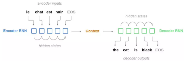
图5.24: seq2seq 模型
▌sequence to sequence 模型
sequence to sequence 模型,或者说seq2seq 模型,由两个RNN 组成。这两个RNN分别叫做encoder 和decoder。encoder 会一个词一个出的读入输入序列,每一步都有一个输出,而最后的输出叫做context 向量,我们可以认为是模型对源语言句子“语义”的一种表示。而decoder 用这个context 向量一步一步的生成目标语言的句子。
为什么要两个RNN 呢,如果我们使用一个RNN,输入和输出是一对一的关系(对于分类,我们可以只使用最后一个输出),但是翻译肯定不是一个词对一个词的翻译。当然这只是使用两个RNN 在形式上的方便,从“原理”上来说,人类翻译也是类似的,首先仔细阅读源语句,然后“理解”它,而所谓的“理解”在seq2seq 模型里可以认为encoding 的过程,然后再根据理解,翻译成目标语句。
▌注意力机制(Attention Mechanism)
用一个固定长度的向量来承载输入序列的完整“语义”,不管向量能有多长,都是很困难的事情。
[Bahdanau et al. 等人引入的](https://arxiv.org/abs/1409.0473) ** 注意力机制**试图这样来解决这个问题:我们不依赖于一个固定长度的向量,而是通过“注意”输入的某些部分。在decoer 每一步解码的时候都通过这个机制来选择输入的一部分来重点考虑。这似乎是合乎人类的翻译过程的——我们首先通过一个encoder 大致理解句子的意思(编码到一个定长向量),具体翻译某个词或者短语的时候我们会仔细推敲对应的源语言的词(注意力机制)。
注意力是通过decoder 的另外一个神经网络层来计算的。它的输入是当前输入和上一个时刻的隐状态,输出是一个新的向量,这个向量的长度和输入相同(因为输入是变长的,我们会选择一个最大的长度),这个向量会用softmax 变成“概率”,得到* 注意力权重*,这个权重可以认为需要花费多大的“注意力”到某个输入上,因此我们会用这个权重加权平均encoder 的输出,从而得到一个新的context 向量,这个向量会用来预测当前时刻的输出。
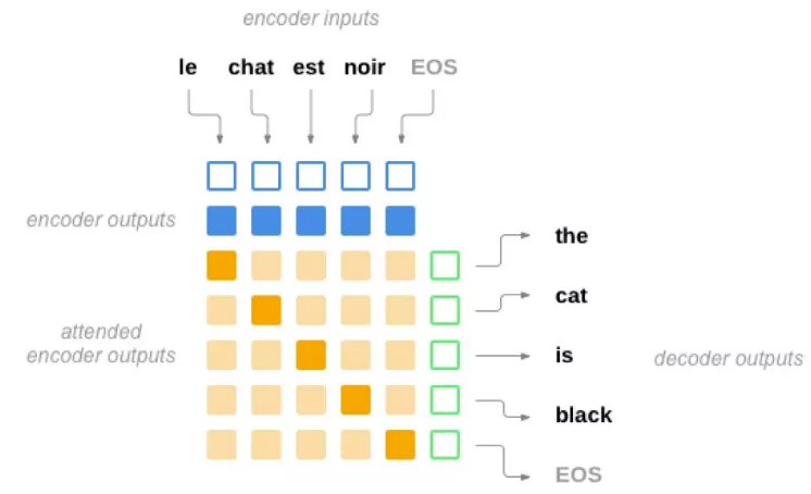
图5.25: 加入注意力机制的Encoder
▌依赖的lib
import unicodedataimport stringimport reimport randomimport timeimport mathimport torchimport torch.nn as nnfrom torch.autograd import Variablefrom torch import optimimport torch.nn.functional as F
是否使用CUDA,这个例子数据较少,所以CPU 也可以训练。
#如果有GPU请改成True
USE_CUDA = False
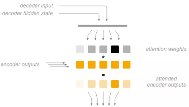
图5.26: 注意力的计算过程
▌加载数据
训练数据是几千个英语到法语的平行句对。我们这里只是介绍算法,所以使用一个很小的数据集来演示。数据在data/eng-fra.txt 里,格式如下:
I am cold. Je suis froid.
我们会用one-hot 的方法来表示一个单词。
1. 单词变成数字
我们会创建一个Lang 对象来表示源/目标语言,它包含word2idx、idx2word 和word2count,分别表示单词到id、id 到单词和单词的词频。word2count 的作用是用于过滤一些低频词(把它变成unknown)
SOS_token = 0
EOS_token = 1
class Lang:
def __init__(self, name):
self.name = name
self.word2index = {}
self.word2count = {}
self.index2word = {0: "SOS", 1: "EOS"}
self.n_words = 2
def index_words(self, sentence):
for word in sentence.split(' '):
self.index_word(word)
def index_word(self, word):
if word not in self.word2index:
self.word2index[word] = self.n_words
self.word2count[word] = 1
self.index2word[self.n_words] = word
self.n_words += 1
else:
self.word2count[word] += 1
def unicode_to_ascii(s):
return ''.join(
c for c in unicodedata.normalize('NFD', s)
if unicodedata.category(c) != 'Mn'
)
# 大小转小写,trim,去掉非字母。
def normalize_string(s):
s = unicode_to_ascii(s.lower().strip())
s = re.sub(r"([.!?])", r" \1", s)
s = re.sub(r"[^a-zA-Z.!?]+", r" ", s)
return s
2. 读取文件
文件格式是每行一个句对,用tab 分隔,第一个是英语,第二个是法语,为了方便未来的复用,我们有一个reverse 参数,这样如果我们需要法语到英语的翻译就可以用到。
def read_langs(lang1, lang2, reverse=False): print("Reading lines...") # 读取文件 lines = open('../data/%s-%s.txt' % (lang1,lang2)).read().strip().split('\n') # split pairs = [[normalize_string(s) for s in l.split('\t')] for l in lines] if reverse: pairs = [list(reversed(p)) for p in pairs] input_lang = Lang(lang2) output_lang = Lang(lang1) else: input_lang = Lang(lang1) output_lang = Lang(lang2) return input_lang, output_lang, pairs
3. 过滤句子
作为演示,我们只挑选长度小于10 的句子,并且这保留”I am” 和”He is” 开头的数据
MAX_LENGTH = 10
good_prefixes = (
"i am ", "i m ",
"he is", "he s ",
"she is", "she s",
"you are", "you re "
)
def filter_pair(p):
return len(p[0].split(' ')) < MAX_LENGTH and len(p[1].split(' ')) < MAX_LENGTH and \
p[1].startswith(good_prefixes)
def filter_pairs(pairs):
return [pair for pair in pairs if filter_pair(pair)]
数据处理过程如下:
• 读取文件,split 成行,再split 成pair
• 文本归一化,通过长度和内容过滤
• 通过pair 里的句子得到单词列表
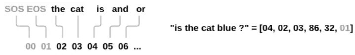
图5.27: 句子变成Tensor
def prepare_data(lang1_name, lang2_name, reverse=False):
input_lang, output_lang, pairs = read_langs(lang1_name, lang2_name,
reverse) print("Read %s sentence pairs" % len(pairs)) pairs = filter_pairs(pairs) print("Trimmed to %s sentence pairs" % len(pairs)) print("Indexing words...") for pair in pairs: input_lang.index_words(pair[0]) output_lang.index_words(pair[1]) return input_lang, output_lang, pairsinput_lang, output_lang, pairs = prepare_data('eng', 'fra', True)print(random.choice(pairs))
▌把训练数据变成Tensor/Variable
为了让神经网络能够处理,我们首先需要把句子变成Tensor。每个句子首先分成词,每个词被替换成对应的index。另外我们会增加一个特殊的EOS 来表示句子的结束。
在PyTorch 里一个Tensor 是一个多维数组,它的所有元素的数据类型都是一样的。我们这里使用LongTensor 来表示词的index。
可以训练的PyTorch 模块要求输入是Variable 而不是Tensor。变量除了包含Tensor 的内容之外,它还会跟踪计算图的状态,从而可以进行自动梯度的求值。
def indexes_from_sentence(lang, sentence):
return [lang.word2index[word] for word in sentence.split(' ')]
def variable_from_sentence(lang, sentence):
indexes = indexes_from_sentence(lang, sentence)
indexes.append(EOS_token)
var = Variable(torch.LongTensor(indexes).view(-1, 1))
if USE_CUDA: var = var.cuda()
return var
def variables_from_pair(pair):
input_variable = variable_from_sentence(input_lang, pair[0])
target_variable = variable_from_sentence(output_lang, pair[1])
return (input_variable, target_variable)
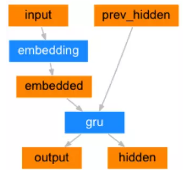
图5.28: Encoder 定义
▌定义模型
1. Encoder
class EncoderRNN(nn.Module):
    def __init__(self, input_size, hidden_size, n_layers=1):
        super(EncoderRNN, self).__init__()

        self.input_size = input_size
        self.hidden_size = hidden_size
        self.n_layers = n_layers

        self.embedding = nn.Embedding(input_size, hidden_size)
        self.gru = nn.GRU(hidden_size, hidden_size, n_layers)

    def forward(self, word_inputs, hidden):
        # 注意:和名字分类不同,我们这里一次处理完一个输入的所有词,而不是for循环每次处理一个词。
        # 两者的效果是一样的,但是一次处理万效率更高。
        seq_len = len(word_inputs)
        embedded = self.embedding(word_inputs).view(seq_len, 1, -1)
        output, hidden = self.gru(embedded, hidden)
        return output, hidden

    def init_hidden(self):
        hidden = Variable(torch.zeros(self.n_layers, 1, self.hidden_size))
        if USE_CUDA: hidden = hidden.cuda()
        return hidden
我们这里的代码每次只处理一个训练句对,这样的实现不是最高效的,但是不要考虑padding,比较容易理解,后面我们会介绍batch 的例子。
2. Attention Decoder
2.1 Bahdanau 等人提出的模型
下面我们来学习一下这篇文章提出的[Neural Machine Translation by JointlyLearning to Align and Translate](https://arxiv.org/abs/1409.0473) Attention Decoder。
decoder 在每一个时刻的输出依赖与前一个时刻的输出和一个x,这个x 包括当前的隐状态(它也会考虑前一个时刻的输出)和一个注意力”context“,下文会介绍它。函数g 是一个带非线性激活的全连接层,它的输入是yi−1, si 和ci 拼接起来的。
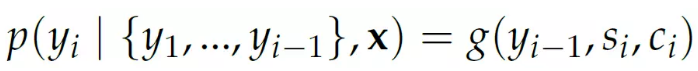
上式的意思是:我们在翻译当前词时只考虑上一个翻译出来的词以及当前的隐状态和注意力context。
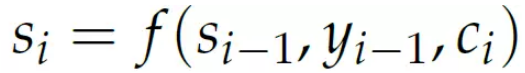
当前隐状态si 是有RNN f 计算出来的,这个RNN 的输入是上一个隐状态si−1,decoder 的上一个输出yi−1 和context 向量ci。
在代码实现中,我们使用的RNN 是‘nn.GRU‘,隐状态si 是‘hidden‘,输出yi是‘output‘,context ci 是‘context‘。
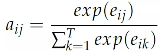
context 向量ci 是encoder 在每个时刻(词) 的输出的加权和,而权值aij 表示i时刻需要关注hj 的程度(概率)。
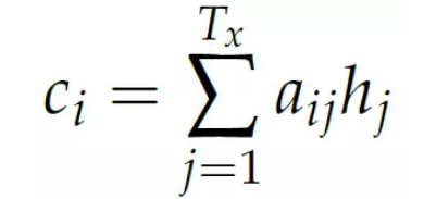
而权值aij 是” 能量” eij 的softmax。
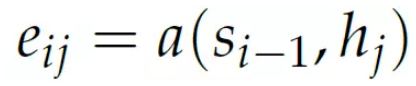
而能量eij 是上个时刻的隐状态si−1 和encoder 第j 个时刻的输出hj 的函数:
2.2 实现Bahdanau 模型
总结一下,我们的decoder 有4 个主要的部分——一个embedding 层用于把输入词变成向量;一个用于计算注意力能量的层;一个RNN 层;一个输出层。
decoder 的输入是上一个时刻的隐状态si−1,上一个时刻的输出yi−1 和所有encoder 的输出h∗。
• embedding 层其输入是上一个时刻的输出yi−1
embedded = embedding(last_rnn_output)
• attention 层首先根据函数a 计算e,其输入是(si−1, hj) 输出是eij,最后对e 用softmax 得到aij
attn_energies[j] = attn_layer(last_hidden, encoder_outputs[j])
attn_weights = normalize(attn_energies)
• context 向量ci 是encoder 的所有时刻的输出的加权和
context = sum(attn_weights * encoder_outputs)
• RNN 层f 的输入是(si−1, yi−1, ci) 和内部的隐状态,输出是si
rnn_input = concat(embedded, context)
rnn_output, rnn_hidden = rnn(rnn_input, last_hidden)
• 输出层g 的输入是(yi−1, si, ci),输出是yi
output = out(embedded, rnn_output, context)
# 注意:我们后面并没有用到这个模型,代码只是为了让读者更加理解前面的内容。class BahdanauAttnDecoderRNN(nn.Module): def __init__(self, hidden_size, output_size, n_layers=1, dropout_p=0.1): super(AttnDecoderRNN, self).__init__() # 定义参数 self.hidden_size = hidden_size self.output_size = output_size self.n_layers = n_layers self.dropout_p = dropout_p self.max_length = max_length # 定义网络 self.embedding = nn.Embedding(output_size, hidden_size) self.dropout = nn.Dropout(dropout_p) self.attn = GeneralAttn(hidden_size) self.gru = nn.GRU(hidden_size * 2, hidden_size, n_layers, dropout=dropout_p) self.out = nn.Linear(hidden_size, output_size) def forward(self, word_input, last_hidden, encoder_outputs): # 每次decode我们只运行一个time step,但是会使用encoder的所有输出 # 得到当前词(decoder的上一个输出)的embedding word_embedded = self.embedding(word_input).view(1, 1, -1) # S=1 x B x N word_embedded = self.dropout(word_embedded) # 计算attention weights attn_weights = self.attn(last_hidden[-1], encoder_outputs) context = attn_weights.bmm(encoder_outputs.transpose(0, 1)) # B x 1 x N # 把word_embedded和context拼接起来作为rnn的输入 rnn_input = torch.cat((word_embedded, context), 2) output, hidden = self.gru(rnn_input, last_hidden) # 输出层 output = output.squeeze(0) # B x N output = F.log_softmax(self.out(torch.cat((output, context), 1)), 1) # 返回结果 return output, hidden, attn_weights
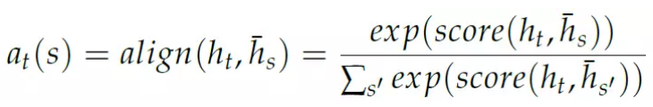
2.3 Luong 等人提出的模型
Luong 等人在[Effective Approaches to Attention-based Neural Machine Translation](https://arxiv.org/abs/1508.04025) 提出了更多的提高和简化。他们描述了”全局注意力“模型,其计算注意力得分的方法和之前不同。前面是通过si−1 和hj 计算aij,也就是当前的注意力权重依赖与前一个状态,而这里的注意力依赖与decoder 当前的隐状态和encoder 所有隐状态:
特点的”score” 函数会比较两个隐状态的”相似度“,可以是两个向量的内积,也可以是hs′ 做一个线性变换之后和ht 的内积,也可以是把两个向量拼接起来然后做一个线性变换,然后和一个参数va(这个参数是学习出来的)的内积:
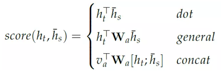
scoring 函数的模块化定义使得我们可以随意的修改而不影响其它地方的代码。
这个模块的输入总是decoder 的隐状态和encoder 的所有输出。
class Attn(nn.Module):
def __init__(self, method, hidden_size, max_length=MAX_LENGTH):
super(Attn, self).__init__()
self.method = method
self.hidden_size = hidden_size
if self.method == 'general':
self.attn = nn.Linear(self.hidden_size, hidden_size)
elif self.method == 'concat':
self.attn = nn.Linear(self.hidden_size * 2, hidden_size)
self.other = nn.Parameter(torch.FloatTensor(1, hidden_size))
def forward(self, hidden, encoder_outputs):
seq_len = len(encoder_outputs)
# 创建变量来存储注意力能量
attn_energies = Variable(torch.zeros(seq_len))
if USE_CUDA: attn_energies = attn_energies.cuda()
# 计算
for i in range(seq_len):
attn_energies[i] = self.score(hidden, encoder_outputs[i])
return F.softmax(attn_energies, 0).unsqueeze(0).unsqueeze(0)
def score(self, hidden, encoder_output):
if self.method == 'dot':
energy = hidden.dot(encoder_output)
return energy
elif self.method == 'general':
energy = self.attn(encoder_output)
energy = hidden.dot(energy)
return energy
elif self.method == 'concat':
energy = self.attn(torch.cat((hidden, encoder_output), 1))
energy = self.other.dot(energy)
return energy
现在我们可以构建一个decoder,它会把Attn 模块放到RNN 之后用来计算注意力的权重,并且用它来计算context 向量。
class AttnDecoderRNN(nn.Module): def __init__(self, attn_model, hidden_size, output_size, n_layers=1, dropout_p=0.1): super(AttnDecoderRNN, self).__init__() # 保存到self里 self.attn_model = attn_model self.hidden_size = hidden_size self.output_size = output_size self.n_layers = n_layers self.dropout_p = dropout_p # 定义网络中的层 self.embedding = nn.Embedding(output_size, hidden_size) self.gru = nn.GRU(hidden_size * 2, hidden_size, n_layers, dropout=dropout_p) self.out = nn.Linear(hidden_size * 2, output_size) # 选择注意力模型 if attn_model != 'none': self.attn = Attn(attn_model, hidden_size) def forward(self, word_input, last_context, last_hidden, encoder_outputs): # 注意:每次我们处理一个time step # 得到当前输入(上一个输出)的embedding word_embedded = self.embedding(word_input).view(1, 1, -1) # S=1 x B x N # 把当前的embedding和上一个context拼接起来输入到RNN里 rnn_input = torch.cat((word_embedded, last_context.unsqueeze(0)), 2) rnn_output, hidden = self.gru(rnn_input, last_hidden) # 使用RNN的输出和所有encoder的输出来计算注意力权重,然后计算context向量 attn_weights = self.attn(rnn_output.squeeze(0), encoder_outputs) context = attn_weights.bmm(encoder_outputs.transpose(0, 1)) # B x 1 x N # 使用RNN的输出和context向量预测下一个词 rnn_output = rnn_output.squeeze(0) # S=1 x B x N -> B x N context = context.squeeze(1) # B x S=1 x N -> B x N output = F.log_softmax(self.out(torch.cat((rnn_output, context), 1)), 1) return output, context, hidden, attn_weights
▌测试代码
为了验证代码是否有问题,我们可以用fake 的数据来测试一下它的输出:
USE_CUDA=False #如果有GPU,改成True
encoder_test = EncoderRNN(10, 10, 2)
decoder_test = AttnDecoderRNN('general', 10, 10, 2)
print(encoder_test)
print(decoder_test)
encoder_hidden = encoder_test.init_hidden()
word_input = Variable(torch.LongTensor([1, 2, 3]))
if USE_CUDA:
encoder_test.cuda()
word_input = word_input.cuda()
encoder_outputs, encoder_hidden = encoder_test(word_input, encoder_hidden)
word_inputs = Variable(torch.LongTensor([1, 2, 3]))
decoder_attns = torch.zeros(1, 3, 3)
decoder_hidden = encoder_hidden
decoder_context = Variable(torch.zeros(1, decoder_test.hidden_size))
if USE_CUDA:
decoder_test.cuda()
word_inputs = word_inputs.cuda()
decoder_context = decoder_context.cuda()
for i in range(3):
decoder_output, decoder_context, decoder_hidden, decoder_attn = decoder_test(word_inputs[i], decoder_context, decoder_hidden, encoder_outputs)
print(decoder_output.size(), decoder_hidden.size(), decoder_attn.size())
decoder_attns[0, i] = decoder_attn.squeeze(0).cpu().data
EncoderRNN(
(embedding): Embedding(10, 10)
(gru): GRU(10, 10, num_layers=2)
)
AttnDecoderRNN(
(embedding): Embedding(10, 10)
(gru): GRU(20, 10, num_layers=2, dropout=0.1)
(out): Linear(in_features=20, out_features=10)
(attn): Attn(
(attn): Linear(in_features=10, out_features=10)
)
)
torch.Size([1, 10]) torch.Size([2, 1, 10]) torch.Size([1, 1, 3])
torch.Size([1, 10]) torch.Size([2, 1, 10]) torch.Size([1, 1, 3])
torch.Size([1, 10]) torch.Size([2, 1, 10]) torch.Size([1, 1, 3])
▌训练代码
1. 一次训练
对于一个训练数据,我们首先用encoder 对输入句子进行编码,得到每个时刻的输出和最后一个时刻的隐状态。最后一个隐状态会作为decoder 隐状态的初始值,并且我们会用一个特殊的<SOS> 作为decoder 的第一个输入。
2. Teacher Forcing 和Scheduled Sampling
”Teacher Forcing”,或者叫最大似然采样,使用目标语言的实际输出来作为decoder 的输入。而另外一种方法就是使用decoder 上一个时刻的输出来作为当前时刻的输入。前者可以让网络更快收敛,但是根据这篇论文(http://minds.jacobs-university.de/sites/default/files/uploads/papers/ESNTutorialRev.pdf),它可能不稳定。
实践中发现,Teacher Forcing 可以学到合法语法的翻译,但是效果很不好。
解决方法是Scheduled Sampling(https://arxiv.org/abs/1506.03099),随机的使用目标语言的输出和decoder 预测的输出。
teacher_forcing_ratio = 0.5clip = 5.0def train(input_variable, target_variable, encoder, decoder, encoder_optimizer, decoder_optimizer, criterion, max_length=MAX_LENGTH): # 梯度清零 encoder_optimizer.zero_grad() decoder_optimizer.zero_grad() loss = 0 # 得到输入和输出句子的长度 input_length = input_variable.size()[0] target_length = target_variable.size()[0] # encoding encoder_hidden = encoder.init_hidden() encoder_outputs, encoder_hidden = encoder(input_variable, encoder_hidden) # 准备输入和输出变量 decoder_input = Variable(torch.LongTensor([[SOS_token]])) decoder_context = Variable(torch.zeros(1, decoder.hidden_size)) decoder_hidden = encoder_hidden # Use last hidden state from encoder to start decoder if USE_CUDA: decoder_input = decoder_input.cuda() decoder_context = decoder_context.cuda() # 随机选择是否Teacher Forcing use_teacher_forcing = random.random() < teacher_forcing_ratio if use_teacher_forcing: # Teacher forcing:使用真实的输出作为下一个时刻的输入 for di in range(target_length): decoder_output, decoder_context, decoder_hidden, decoder_attention = decoder(decoder_input, decoder_context, decoder_hidden, encoder_outputs) loss += criterion(decoder_output, target_variable[di]) decoder_input = target_variable[di] # 下一个时刻的输入来自target else: # 不使用 teacher forcing:使用decoder的预测作为下一个时刻的输入 for di in range(target_length): decoder_output, decoder_context, decoder_hidden, decoder_attention = decoder(decoder_input, decoder_context, decoder_hidden, encoder_outputs) loss += criterion(decoder_output, target_variable[di]) # 选择最可能的词 topv, topi = decoder_output.data.topk(1) ni = topi[0][0] decoder_input = Variable(torch.LongTensor([[ni]])) # 下个时刻的输入 if USE_CUDA: decoder_input = decoder_input.cuda() # 如果decoder输出EOS_token,那么提前结束 if ni == EOS_token: break # 反向计算梯度 loss.backward() torch.nn.utils.clip_grad_norm(encoder.parameters(), clip) torch.nn.utils.clip_grad_norm(decoder.parameters(), clip) encoder_optimizer.step() decoder_optimizer.step() return loss.data[0] / target_length
▌训练
所有准备工作都好了,我们可以初始化网络并开始训练了。
我们首先初始化网络,优化器和损失函数
attn_model = 'general'
hidden_size = 500
n_layers = 2
dropout_p = 0.05
# 初始化模型
encoder = EncoderRNN(input_lang.n_words, hidden_size, n_layers)
decoder = AttnDecoderRNN(attn_model, hidden_size, output_lang.n_words, n_layers, dropout_p=dropout_p)
# 把变量放到GPU里
if USE_CUDA:
encoder.cuda()
decoder.cuda()
# 初始化optimizer和criterion,注意:我们这里用两个optimizer分别来优化encoder和decoder的参数。
learning_rate = 0.0001
encoder_optimizer = optim.Adam(encoder.parameters(), lr=learning_rate)
decoder_optimizer = optim.Adam(decoder.parameters(), lr=learning_rate)
criterion = nn.NLLLoss()
定义一些变量用于保存历史的loss
# 训练的一些超参数n_epochs = 50000plot_every = 200print_every = 1000# 保存开始时间和lossstart = time.time()plot_losses = []print_loss_total = 0plot_loss_total = 0
开始训练:
for epoch in range(1, n_epochs + 1):
# 得到一个训练句对
training_pair = variables_from_pair(random.choice(pairs))
input_variable = training_pair[0]
target_variable = training_pair[1]
# 训练一次
loss = train(input_variable, target_variable, encoder, decoder,
encoder_optimizer, decoder_optimizer, criterion)
print_loss_total += loss
plot_loss_total += loss
if epoch == 0: continue
if epoch % print_every == 0:
print_loss_avg = print_loss_total / print_every
print_loss_total = 0
print_summary = '%s (%d %d%%) %.4f' % (time_since(start, epoch /
n_epochs), epoch, epoch / n_epochs * 100, print_loss_avg)
print(print_summary)
if epoch % plot_every == 0:
plot_loss_avg = plot_loss_total / plot_every
plot_losses.append(plot_loss_avg)
plot_loss_total = 0
▌训练loss 绘图
import matplotlib.pyplot as pltimport matplotlib.ticker as tickerimport numpy as np%matplotlib inlinedef show_plot(points): plt.figure() fig, ax = plt.subplots() loc = ticker.MultipleLocator(base=0.2) ax.yaxis.set_major_locator(loc) plt.plot(points)show_plot(plot_losses)
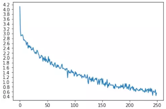
图5.29: 损失变化图
▌评估效果
实际翻译的代码和训练类似,我们用上一个时刻的输出作为下一个时刻的输入,当遇到EOS 时我们认为翻译结束。
def evaluate(sentence, max_length=MAX_LENGTH):
input_variable = variable_from_sentence(input_lang, sentence)
input_length = input_variable.size()[0]
encoder_hidden = encoder.init_hidden()
encoder_outputs, encoder_hidden = encoder(input_variable, encoder_hidden)
decoder_input = Variable(torch.LongTensor([[SOS_token]])) # SOS
decoder_context = Variable(torch.zeros(1, decoder.hidden_size))
if USE_CUDA:
decoder_input = decoder_input.cuda()
decoder_context = decoder_context.cuda()
decoder_hidden = encoder_hidden
decoded_words = []
decoder_attentions = torch.zeros(max_length, max_length)
for di in range(max_length):
decoder_output, decoder_context, decoder_hidden, decoder_attention = decoder(decoder_input, decoder_context, decoder_hidden, encoder_outputs)
decoder_attentions[di,:decoder_attention.size(2)] += decoder_attention.squeeze(0).squeeze(0).cpu().data
topv, topi = decoder_output.data.topk(1)
ni = topi[0][0]
if ni == EOS_token:
decoded_words.append('<EOS>')
break
else:
decoded_words.append(output_lang.index2word[ni])
# Next input is chosen word
decoder_input = Variable(torch.LongTensor([[ni]]))
if USE_CUDA: decoder_input = decoder_input.cuda()
return decoded_words, decoder_attentions[:di+1, :len(encoder_outputs)]
我们来测试一下效果:
def evaluate_randomly(): pair = random.choice(pairs) output_words, decoder_attn = evaluate(pair[0]) output_sentence = ' '.join(output_words) print('>', pair[0]) print('=', pair[1]) print('<', output_sentence) print('')evaluate_randomly()
结果:
> il est irrealiste .
= he is unrealistic .
< he s out . <EOS>
▌注意力的可视化
注意力可以看出一种soft 的对齐,我们可以观察模型怎么”对齐“源语言的词和目标语言的词。
def show_attention(input_sentence, output_words, attentions): # Set up figure with colorbar fig = plt.figure() ax = fig.add_subplot(111) cax = ax.matshow(attentions.numpy(), cmap='bone') fig.colorbar(cax) # Set up axes ax.set_xticklabels([''] + input_sentence.split(' ') + ['<EOS>'], rotation=90) ax.set_yticklabels([''] + output_words) # Show label at every tick ax.xaxis.set_major_locator(ticker.MultipleLocator(1)) ax.yaxis.set_major_locator(ticker.MultipleLocator(1)) plt.show() plt.close()def evaluate_and_show_attention(input_sentence): output_words, attentions = evaluate(input_sentence) print('input =', input_sentence) print('output =', ' '.join(output_words)) show_attention(input_sentence, output_words, attentions)
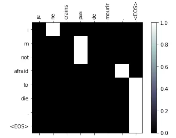
图5.30: Attention 的翻译对齐
汉语-英语翻译的批量训练
前面我们介绍了基本的seq2seq 模型,Attention 机制,但是它每次只能训练一个句对,因此训练的速度是个问答,读者可以尝试一下加入更多数据时的训练速度。本节我们介绍怎么一次训练一个batch 的数据,从而加速训练。我们会使用汉语到英语的数据来实现一个简单汉-英翻译系统。大致的代码和前面是类似的,我们下面着重介绍其中不同的地方,完整的代码请读者参考
https://github.com/fancyerii/deep_learning_theory_and_practice/blob/master/codes/ch05/seq2seq-translation-batched-cn-fixbug.ipynb
▌数据处理
中文和法语不同的地方就是不能通过空格来分词,我们这里已经提前分好词并用空格分开了。训练数据在:
https://github.com/fancyerii/deep_learning_theory_and_practice/
blob/master/codes/data/eng-chn.txt。
数据格式为每行一个句对,格式是“英语句子tab 汉语句子”。
此外,我们还会去掉频率较低的词已经包含低频词的句对。所以类Lang 会增加一个trim 方法:
PAD_token = 0
SOS_token = 1
EOS_token = 2
class Lang:
def __init__(self, name):
self.name = name
self.trimmed = False
self.word2index = {}
self.word2count = {}
self.index2word = {0: "PAD", 1: "SOS", 2: "EOS"}
self.n_words = 3 # Count default tokens
def seg_words(self, sentence):
return sentence.split(' ')
def index_words(self, sentence):
words=self.seg_words(sentence)
for word in words:
self.index_word(word)
def index_word(self, word):
if word not in self.word2index:
self.word2index[word] = self.n_words
self.word2count[word] = 1
self.index2word[self.n_words] = word
self.n_words += 1
else:
self.word2count[word] += 1
# 删除掉频率少于阈值的此。
def trim(self, min_count):
if self.trimmed: return
self.trimmed = True
keep_words = []
for k, v in self.word2count.items():
if v >= min_count:
keep_words.append(k)
print('keep_words %s / %s = %.4f' % (
len(keep_words), len(self.word2index), len(keep_words) /
len(self.word2index)
))
# 重新构建dict
self.word2index = {}
self.word2count = {}
self.index2word = {0: "PAD", 1: "SOS", 2: "EOS"}
self.n_words = 3 # 默认3个词。
for word in keep_words:
self.index_word(word)
这里我们会滤掉过短(小于3) 或者过长(大于25) 的句对:
MIN_LENGTH = 3MAX_LENGTH = 25def filter_pairs(pairs):filtered_pairs = []for pair in pairs: if len(pair[0]) >= MIN_LENGTH and len(pair[0]) <= MAX_LENGTH \ and len(pair[1]) >= MIN_LENGTH and len(pair[1]) <= MAX_LENGTH: filtered_pairs.append(pair)return filtered_pairs
过滤完成后,我们只剩下1854 个中英句对,我们可以查看其中的一个:
print(pairs[2])
['我赢了。', 'i won !']
▌Padding
为了更好的使用GPU,我们一次训练一个batch 的数据,但是问题是不同句对的长度是不一样的。解决办法是通过“pad”来把短的序列补到和长的序列一样长,我们需要一个特殊的整数来表示它是一个pad 值而不是其他的词,我们这里使用0。当计算loss 的时候,我们也需要把这些0 对应的loss 去掉(因为实际的序列到这里已经没有了,但是padding 之后任何会计算出模型的预测值,从而有loss)
padding 如图5.31所示。padding 的代码如下:
# 把一个序列padding到长度为max_length。def pad_seq(seq, max_length): seq += [PAD_token for i in range(max_length - len(seq))] return seq
▌随机选择一个batch 的训练数据
训练一次需要一个batch 的数据,我们一般随机的抽取bach_size 个句对,然后把它们padding 到最长的序列长度。此外,我们需要记录下未padding 之前的长度,因为计算loss 的时候会需要用到它。
我们会用list 的list 来初始化LongTensor,这个list 的大小是batch_size,list的每个元素是一个序列(句子)。这样我们可以得到一个(batch_size x max_len) 的Tensor,但是因为训练时我们需要逐个时刻的计算batch_size 个数据,所以我们需要把它转置成(max_len x batch_size)。这样tensor[t] 就表示t 时刻的batch_size 个词,转置过程如图5.32所示。
随机选择batch_size 个数据的代码:
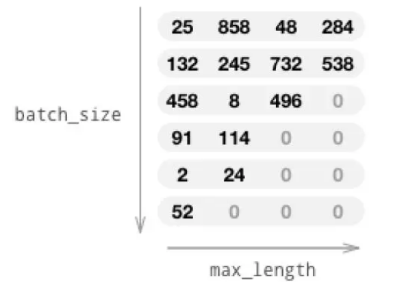
图5.31: Padding
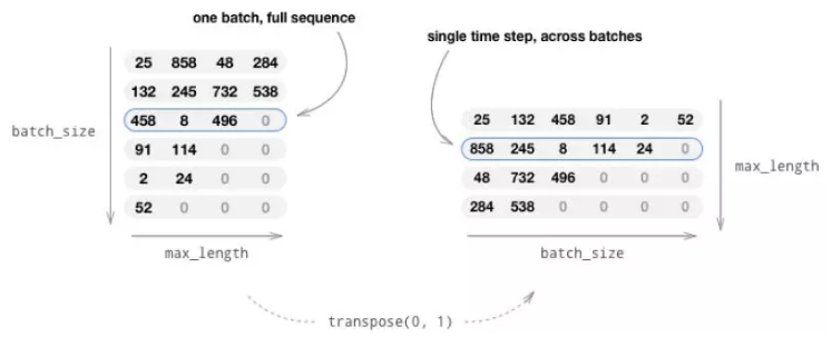
图5.32: 转置
def random_batch(batch_size):
input_seqs = []
target_seqs = []
# 随机选择pairs
for i in range(batch_size):
pair = random.choice(pairs)
input_seqs.append(indexes_from_sentence(input_lang, pair[0]))
target_seqs.append(indexes_from_sentence(output_lang, pair[1]))
# 把输入和输出序列zip起来,通过输入的长度降序排列,然后unzip
seq_pairs = sorted(zip(input_seqs, target_seqs), key=lambda p: len(p[0]),
reverse=True)
input_seqs, target_seqs = zip(*seq_pairs)
# 对输入和输出序列都进行padding。
input_lengths = [len(s) for s in input_seqs]
input_padded = [pad_seq(s, max(input_lengths)) for s in input_seqs]
target_lengths = [len(s) for s in target_seqs]
target_padded = [pad_seq(s, max(target_lengths)) for s in target_seqs]
# padding之后的shape是(batch_size x max_len),我们需要把它转置成(max_len x
batch_size)
input_var = Variable(torch.LongTensor(input_padded)).transpose(0, 1)
target_var = Variable(torch.LongTensor(target_padded)).transpose(0, 1)
if USE_CUDA:
input_var = input_var.cuda()
target_var = target_var.cuda()
return input_var, input_lengths, target_var, target_lengths
▌定义模型
1. Encoder
Encoder 和之前的版本类似,不过这里我们使用两层双向的GRU。
class EncoderRNN(nn.Module): def __init__(self, input_size, hidden_size, n_layers=1, dropout=0.1): super(EncoderRNN, self).__init__() self.input_size = input_size self.hidden_size = hidden_size self.n_layers = n_layers self.dropout = dropout self.embedding = nn.Embedding(input_size, hidden_size) self.gru = nn.GRU(hidden_size, hidden_size, n_layers, dropout=self.dropout, bidirectional=True) def forward(self, input_seqs, input_lengths, hidden=None): # 注意:和前面的实现不同,这里没有时刻t的for循环,而是一次输入GRU直接计算出来 embedded = self.embedding(input_seqs) packed = torch.nn.utils.rnn.pack_padded_sequence(embedded, input_lengths) outputs, hidden = self.gru(packed, hidden) outputs, output_lengths = torch.nn.utils.rnn.pad_packed_sequence(outputs) # unpackhidden = self._cat_directions(hidden)return outputs, hidden def _cat_directions(self, hidden): """ 双向的encoder,我们需要把双向的结果拼接起来。----------------------------------------------------------- In: (num_layers * num_directions, batch_size, hidden_size) (ex: num_layers=2, num_directions=2) layer 1: forward__hidden(1) layer 1: backward_hidden(1) layer 2: forward__hidden(2) layer 2: backward_hidden(2)----------------------------------------------------------- Out: (num_layers, batch_size, hidden_size * num_directions) layer 1: forward__hidden(1) backward_hidden(1) layer 2: forward__hidden(2) backward_hidden(2) """ def _cat(h): return torch.cat([h[0:h.size(0):2], h[1:h.size(0):2]], 2) if isinstance(hidden, tuple): # LSTM hidden contains a tuple (hidden state, cell state) hidden = tuple([_cat(h) for h in hidden]) else: # GRU hidden hidden = _cat(hidden)return hidden
在__init__ 方法里,它和之前不同的地方就是GRU 的bidirectional 是True,并且传入层数n_layers。
而forward 方法里,embedding 之后,我们把embedded 和input_lengths 通过torch.nn.utils.rnn.pack_padded_sequence 函数把padding 后的数据和padding 前的长度封装成PackedSequence 对象。这样把它传给GRU 后,GRU 就能知道每个序列的真正长度,这样它返回的hidden_state 就是实际的最后一个时刻的隐状态,而不是padding 了0 之后的最大时刻的隐状态。【当然GRU 的输出是一个Tensor,所以返回的输出包括了padding 后的,因此计算Loss 的时候我们需要去掉padding 时刻的loss,后面会讲到】把packed 和hidden 传入gru 之后,会得到outputs 和最终的隐状态hidden,hidden 后面我们会详细介绍。outputs 是一个PackedSequence 对象,我们可以用pad_packed_sequence 得到最终的输出(包含padding)outputs 和它的长度output_lengths【它和input_lengths 应该是一样的】。
回忆一下,我们会把encoder 的最后时刻的隐状态作为decoder 的输入,如果encoder 是两层的,那么decoder 也应该是两层的,并且要求它们的隐单元的个数也是一样的。但是这里有一个问题:encoder 可以是双向的,因为输入是给定的,但是decoder 的时候(尤其是预测的时候),由于需要要前一个时刻的输出作为下一个时刻的输入,因此不可能是双向的GRU。举个例子,假设输入是两层的双向的GRU,每个有128 个隐单元,那么最后时刻的隐状态也有两层,每层包括128 个forward 的隐状态和128 个backward 的隐状态。
decoder 首先也得是两层的GRU,但是必须是单向的(读者请思考为什么?)。
它的隐单元个数是256,这样我们可以把encoder 的最后一个正向结果和最后一个(第一个时刻) 逆向结果拼接成一个256 的向量传给decoder。代码hidden =self._cat_directions(hidden) 就是实现了把encoder 的双向结果拼接在一起。我们下面来分析这个函数。
我们以GRU 为例,我们假设它是两层的双向GRU,那么调用outputs, hidden= self.gru(packed, hidden) 之后,outputs 的大小是(seq_len, batch, hidden_size *num_directions=256)。而hidden 的大小是(num_layers * num_directions, batch,hidden_size)=(4, batch, 128)。我们先忽略batch(认为它是1),那么它是4 个128 维的向量,分别表示第一层正向的最后一个隐状态;第一层逆向的最后一个隐状态;第二层正向的最后一个隐状态,第二次逆向的最后一个隐状态。现在我们需要把第一层的正向逆向拼接以及第二层的正向逆向拼接,因此torch.cat([h[0:h.size(0):2],h[1:h.size(0):2]], 2) 就实现了上面的拼接。其中h[0:h.size(0):2] 取出两层的forward 结果,而h[1:h.size(0):2] 取出backward 结果,然后再把它们拼起来。
2. LuongAttnDecoderRNN 和前面相比,Decoder 变化不大,只不过是变成了batch 的输入而已,但是在时间维度还是循环处理的,请读者比较其中的细小区别:
class LuongAttnDecoderRNN(nn.Module):
def __init__(self, attn_model, hidden_size, output_size, n_layers=1,
dropout=0.1):
super(LuongAttnDecoderRNN, self).__init__()
# 保存变量
self.attn_model = attn_model
self.hidden_size = hidden_size
self.output_size = output_size
self.n_layers = n_layers)
self.dropout = dropout
# 定义网络层
self.embedding = nn.Embedding(output_size, hidden_size)
self.embedding_dropout = nn.Dropout(dropout)
self.gru = nn.GRU(hidden_size, hidden_size, n_layers, dropout=dropout)
self.concat = nn.Linear(hidden_size * 2, hidden_size)
self.out = nn.Linear(hidden_size, output_size)
# 选择注意力计算方法
if attn_model != 'none':
self.attn = Attn(attn_model, hidden_size)
def forward(self, input_seq, last_hidden, encoder_outputs):
#
注意:我们encoder一次计算所有时刻的数据,但是decoder我们目前还是一次计算一个时刻的(但
# 因为Teacher Forcing可以一次计算但是Random Sample必须逐个计算
# 得到当前输入的embedding
batch_size = input_seq.size(0)
embedded = self.embedding(input_seq)
embedded = self.embedding_dropout(embedded)
embedded = embedded.view(1, batch_size, self.hidden_size) # S=1 x B x N
# 计算gru的输出和新的隐状态,输入是当前词的embedding和之前的隐状态。
rnn_output, hidden = self.gru(embedded, last_hidden)
# 根据当前的RNN状态和encoder的输出计算注意力。
# 根据注意力计算context向量
attn_weights = self.attn(rnn_output, encoder_outputs)
context = attn_weights.bmm(encoder_outputs.transpose(0, 1)) # B x S=1 x
N
# 把gru的输出和context vector拼接起来
rnn_output = rnn_output.squeeze(0) # S=1 x B x N -> B x N
context = context.squeeze(1) # B x S=1 x N -> B x N
concat_input = torch.cat((rnn_output, context), 1)
concat_output = F.tanh(self.concat(concat_input))
# 预测下一个token,这里没有softmax,只有计算loss的时候才需要。
output = self.out(concat_output)
# 返回最终的输出,GRU的隐状态和attetion(用于可视化)
return output, hidden, attn_weights
▌训练
训练的代码和之前没有太多区别。
▌测试结果
如图5.33所示,我们发现它确实学会了中文和英文的词的对应关系。我们会发现大部分情况下中英文的词都是对齐的,但是最后一个中文标点(比如句号)除了对齐英文标点外还把EOS 对齐了。原因可能是在训练数据中最后一个中文标点的后面出现的都是EOS,所以它学到的就是最后一个中文标点就翻译成EOS。
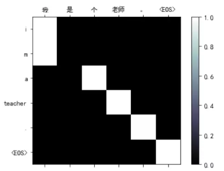
图5.33: 翻译样例
未完待续
关注人工智能头条,获取更多技术干货