TensorFlow学习笔记2："Hello World!"

本文参考TF官方入门程序链接：
https://tensorflow.google.cn/tutorials/keras/basic_classification
推荐直接看以上链接中的官方教程，如果无法打开该链接可以直接看以下内容，以下为官方内容的一个搬运，以保证本系列的完整性，便于自己学习使用。
本教程会训练一个对服饰（例如运动鞋和衬衫）图像进行分类的神经网络模型。
本教程使用 tf.keras，它是一种用于在 TensorFlow 中构建和训练模型的高阶 API。

# TensorFlow and tf.keras
import tensorflow as tf
from tensorflow import keras

# Helper libraries
import numpy as np
import matplotlib.pyplot as plt

print(tf.__version__)

1.12.0

**

（1）导入 Fashion MNIST 数据集

**
本教程使用 Fashion MNIST 数据集，其中包含 70000 张灰度图像，涵盖 10 个类别。以下图像显示了单件服饰在较低分辨率（28x28 像素）下的效果：

Fashion MNIST 的作用是成为经典 MNIST 数据集的简易替换，后者通常用作计算机视觉机器学习程序的“Hello, World”入门数据集。MNIST 数据集包含手写数字（0、1、2 等）的图像，这些图像的格式与我们在本教程中使用的服饰图像的格式相同。
本教程使用 Fashion MNIST 实现多样化，并且它比常规 MNIST 更具挑战性。这两个数据集都相对较小，用于验证某个算法能否如期正常运行。它们都是测试和调试代码的良好起点。

我们将使用 60000 张图像训练网络，并使用 10000 张图像评估经过学习的网络分类图像的准确率。我们可以从 TensorFlow 直接访问 Fashion MNIST，只需导入和加载数据即可：

fashion_mnist = keras.datasets.fashion_mnist

(train_images, train_labels), (test_images, test_labels) = fashion_mnist.load_data()

Downloading data from https://storage.googleapis.com/tensorflow/tf-keras-datasets/train-labels-idx1-ubyte.gz
32768/29515 [=================================] - 0s 0us/step
Downloading data from https://storage.googleapis.com/tensorflow/tf-keras-datasets/train-images-idx3-ubyte.gz 
26427392/26421880 [==============================] - 1s 0us/step 
Downloading data from https://storage.googleapis.com/tensorflow/tf-keras-datasets/t10k-labels-idx1-ubyte.gz 
8192/5148 [===============================================] - 0s 0us/step 
Downloading data from https://storage.googleapis.com/tensorflow/tf-keras-datasets/t10k-images-idx3-ubyte.gz
4423680/4422102 [==============================] - 0s 0us/step

加载数据集会返回 4 个 NumPy 数组：

• train_images 和 train_labels 数组是训练集，即模型用于学习的数据。
• 测试集 test_images 和 test_labels 数组用于测试模型。

图像为 28x28 的 NumPy 数组，像素值介于 0 到 255 之间。标签是整数数组，介于 0 到 9 之间。这些标签对应于图像代表的服饰所属的类别：

标签	类别
0	T 恤衫/上衣
1	裤子
2	套衫
3	裙子
4	外套
5	凉鞋
6	衬衫
7	运动鞋
8	包包
9	踝靴

每张图像都映射到一个标签。由于数据集中不包含类别名称，因此将它们存储在此处，以便稍后在绘制图像表时使用：

class_names = ['T-shirt/top', 'Trouser', 'Pullover', 'Dress', 'Coat',
               'Sandal', 'Shirt', 'Sneaker', 'Bag', 'Ankle boot']

**

（2）观察数据

**
我们先观察数据集的格式，然后再训练模型。以下内容显示训练集中有 60000 张图像，每张图像都表示为 28x28 像素：

print(train_images.shape)

(60000, 28, 28)

同样，训练集中有 60000 个标签：

print(len(train_labels))

 60000

每个标签都是一个介于 0 到 9 之间的整数：

print(train_labels)

 [9, 0, 0, ..., 3, 0, 5]

测试集中有 10000 张图像。同样，每张图像都表示为 28x28 像素：

print(test_images.shape)

 (10000, 28, 28)

测试集中有 10000 个图像标签：

print(len(test_labels))

10000

**

（3）预处理数据

**
必须先对数据进行预处理，然后再训练网络。如果你检查训练集中的第一张图像，就会发现像素值介于 0 到 255 之间：

plt.figure()
plt.imshow(train_images[0])
plt.colorbar()
plt.grid(False)

将这些值缩小到 0 到 1 之间，然后将其馈送到神经网络模型中。为此，将图像组件的数据类型从整数转换为浮点数，然后除以 255。以下是预处理图像的函数：

务必要以相同的方式对训练集和测试集进行预处理：

train_images = train_images / 255.0

test_images = test_images / 255.0

显示训练集中的前 25 张图像，并在每张图像下显示类别名称。验证确保数据格式正确无误，然后我们就可以开始构建和训练网络了。

plt.figure(figsize=(10,10))
for i in range(25):
    plt.subplot(5,5,i+1)
    plt.xticks([])
    plt.yticks([])
    plt.grid(False)
    plt.imshow(train_images[i], cmap=plt.cm.binary)
    plt.xlabel(class_names[train_labels[i]])

**

（4）构建模型

**
构建神经网络需要先配置模型的层，然后再编译模型。

①设置层
神经网络的基本构造块是层。层从馈送到其中的数据中提取表示结果。希望这些表示结果有助于解决手头问题。
大部分深度学习都会把简单的层连在一起。大部分层（例如 tf.keras.layers.Dense）都具有在训练期间要学习的参数。

model = keras.Sequential([
    keras.layers.Flatten(input_shape=(28, 28)),
    keras.layers.Dense(128, activation=tf.nn.relu),
    keras.layers.Dense(10, activation=tf.nn.softmax)
])

该网络中的第一层 tf.keras.layers.Flatten 将图像格式从二维数组（28x28 像素）转换成一维数组（28 * 28 = 784 像素）。可以将该层视为图像中像素未堆叠的行，并排列这些行。该层没有要学习的参数；它只改动数据的格式。

在扁平化像素之后，该网络包含两个 tf.keras.layers.Dense 层的序列。这些层是密集连接或全连接神经层。第一个 Dense 层具有 128 个节点（或神经元）。第二个（也是最后一个）层是具有 10 个节点的 softmax 层，该层会返回一个具有 10 个概率得分的数组，这些得分的总和为 1。每个节点包含一个得分，表示当前图像属于 10 个类别中某一个的概率。

②编译模型
模型还需要再进行几项设置才可以开始训练。这些设置会添加到模型的编译步骤：

• 损失函数 - 衡量模型在训练期间的准确率。我们希望尽可能缩小该函数，以“引导”模型朝着正确的方向优化。
• 优化器 - 根据模型看到的数据及其损失函数更新模型的方式。
• 指标 - 用于监控训练和测试步骤。以下示例使用准确率，即图像被正确分类的比例。

model.compile(optimizer=tf.train.AdamOptimizer(),
              loss='sparse_categorical_crossentropy',
              metrics=['accuracy'])

**

（5）训练模型

**
训练神经网络模型需要执行以下步骤：
1.将训练数据馈送到模型中，在本示例中为 train_images 和 train_labels 数组。
2.模型学习将图像与标签相关联。
3.我们要求模型对测试集进行预测，在本示例中为 test_images 数组。我们会验证预测结果是否与 test_labels 数组中的标签一致。

要开始训练，需要调用 model.fit 方法，使模型与训练数据“拟合”：

model.fit(train_images, train_labels, epochs=5)

Epoch 1/5 60000/60000 [==============================] - 17s 278us/step - loss: 0.4967 - acc: 0.8239 
Epoch 2/5 60000/60000 [==============================] - 10s 174us/step - loss: 0.3715 - acc: 0.8664 
Epoch 3/5 60000/60000 [==============================] - 13s 211us/step - loss: 0.3346 - acc: 0.8785 
Epoch 4/5 60000/60000 [==============================] - 11s 175us/step - loss: 0.3103 - acc: 0.8862 
Epoch 5/5 60000/60000 [==============================] - 10s 159us/step - loss: 0.2942 - acc: 0.8914

在模型训练期间，系统会显示损失和准确率指标。该模型在训练数据上的准确率达到 0.89（即 89%）。
**

（6）评估准确率

**
接下来，比较一下模型在测试数据集上的表现：

test_loss, test_acc = model.evaluate(test_images, test_labels)

print('Test accuracy:', test_acc)

10000/10000 [==============================] - 1s 142us/step
Test accuracy: 0.8775

结果表明，模型在测试数据集上的准确率略低于在训练数据集上的准确率。训练准确率和测试准确率之间的这种差异表示出现过拟合。如果机器学习模型在新数据上的表现不如在训练数据上的表现，就表示出现过拟合。

**

（7）做出预测

**
模型经过训练后，我们可以使用它对一些图像进行预测。

predictions = model.predict(test_images)

在本示例中，模型已经预测了测试集中每张图像的标签。我们来看看第一个预测：

print(predictions[0])

[7.7252298e-07 9.4405972e-10 4.8799400e-08 1.6394343e-07 6.3851907e-08
 6.3104313e-03 1.8902688e-06 2.1339078e-02 1.0463690e-05 9.7233713e-01]

预测结果是一个具有 10 个数字的数组。这些数字说明模型对于图像对应于 10 种不同服饰中每一个服饰的“置信度”。我们可以看到哪个标签的置信度值最大：

print(np.argmax(predictions[0]))

9

因此，模型非常确信这张图像是踝靴或属于 class_names[9]。我们可以检查测试标签以查看该预测是否正确：

print(test_labels[0])

9

我们可以将该预测绘制成图来查看全部 10 个通道

def plot_image(i, predictions_array, true_label, img):
  predictions_array, true_label, img = predictions_array[i], true_label[i], img[i]
  plt.grid(False)
  plt.xticks([])
  plt.yticks([])

  plt.imshow(img, cmap=plt.cm.binary)

  predicted_label = np.argmax(predictions_array)
  if predicted_label == true_label:
    color = 'blue'
  else:
    color = 'red'

  plt.xlabel("{} {:2.0f}% ({})".format(class_names[predicted_label],
                                100*np.max(predictions_array),
                                class_names[true_label]),
                                color=color)

def plot_value_array(i, predictions_array, true_label):
  predictions_array, true_label = predictions_array[i], true_label[i]
  plt.grid(False)
  plt.xticks([])
  plt.yticks([])
  thisplot = plt.bar(range(10), predictions_array, color="#777777")
  plt.ylim([0, 1])
  predicted_label = np.argmax(predictions_array)

  thisplot[predicted_label].set_color('red')
  thisplot[true_label].set_color('blue')

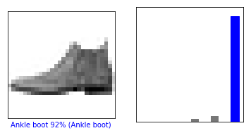
我们来看看第 0 张图像、预测和预测数组。

i = 0
plt.figure(figsize=(6,3))
plt.subplot(1,2,1)
plot_image(i, predictions, test_labels, test_images)
plt.subplot(1,2,2)
plot_value_array(i, predictions,  test_labels)

i = 12
plt.figure(figsize=(6,3))
plt.subplot(1,2,1)
plot_image(i, predictions, test_labels, test_images)
plt.subplot(1,2,2)
plot_value_array(i, predictions,  test_labels)

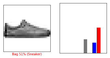
我们用它们的预测绘制几张图像。正确的预测标签为蓝色，错误的预测标签为红色。数字表示预测标签的百分比（总计为 100）。请注意，即使置信度非常高，也有可能预测错误。

# Plot the first X test images, their predicted label, and the true label
# Color correct predictions in blue, incorrect predictions in red
num_rows = 5
num_cols = 3
num_images = num_rows*num_cols
plt.figure(figsize=(2*2*num_cols, 2*num_rows))
for i in range(num_images):
  plt.subplot(num_rows, 2*num_cols, 2*i+1)
  plot_image(i, predictions, test_labels, test_images)
  plt.subplot(num_rows, 2*num_cols, 2*i+2)
  plot_value_array(i, predictions, test_labels)

最后，使用经过训练的模型对单个图像进行预测。

# Grab an image from the test dataset
img = test_images[0]

print(img.shape)

(28, 28)

tf.keras 模型已经过优化，可以一次性对样本批次或样本集进行预测。因此，即使我们使用单个图像，仍需要将其添加到列表中：

# Add the image to a batch where it's the only member.
img = (np.expand_dims(img,0))

print(img.shape)

(1, 28, 28)

现在，预测这张图像：

predictions_single = model.predict(img)

print(predictions_single)

[[7.7252298e-07 9.4405972e-10 4.8799304e-08 1.6394372e-07 6.3852028e-08
  6.3104290e-03 1.8902635e-06 2.1339055e-02 1.0463670e-05 9.7233713e-01]]

plot_value_array(0, predictions_single, test_labels)
_ = plt.xticks(range(10), class_names, rotation=45)

model.predict 返回一组列表，每个列表对应批次数据中的每张图像。（仅）获取批次数据中相应图像的预测结果：

print(np.argmax(predictions_single[0]))

9

和刚才一样，模型预测的标签为 9。
至此"Hello World!"程序结束。

开启新的征程！