在本次分析中,我使用了随机森林回归,并涉及数据标准化和超参数调优。在这里,我使用随机森林分类器,对好酒和不太好的酒进行二元分类。
首先导入数据包:
import numpy as np
import pandas as pd
import matplotlib.pyplot as plt
import seaborn as sns
导入数据:
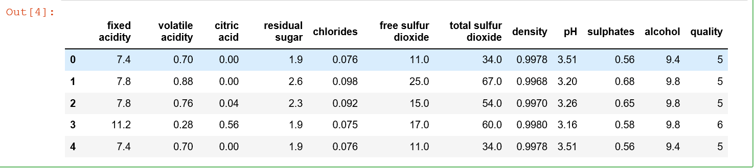
data = pd.read_csv('winequality-red.csv')
data.head()
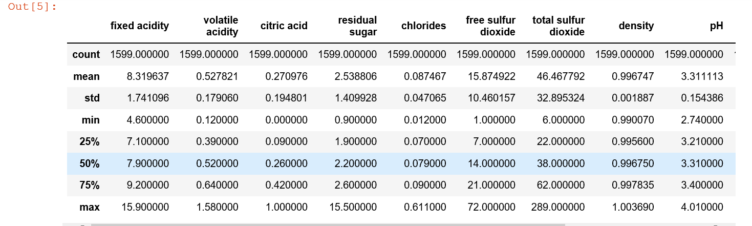
data.describe()
注释:
fixed acidity:非挥发性酸
volatile acidity : 挥发性酸
citric acid:柠檬酸
residual sugar :剩余糖分
chlorides:氯化物
free sulfur dioxide :游离二氧化硫
total sulfur dioxide:总二氧化硫
density:密度
pH:pH
sulphates:硫酸盐
alcohol:酒精
quality:质量
所有数据的数值为1599,所以没有缺失值。让我们看看是否有重复值:
extra = data[data.duplicated()]
extra.shape

有240个重复值,但先不删除它,因为葡萄酒的质量等级是由不同的品酒师给出的。
数据可视化
sns.set()
data.hist(figsize=(10,10), color='red')
plt.show()
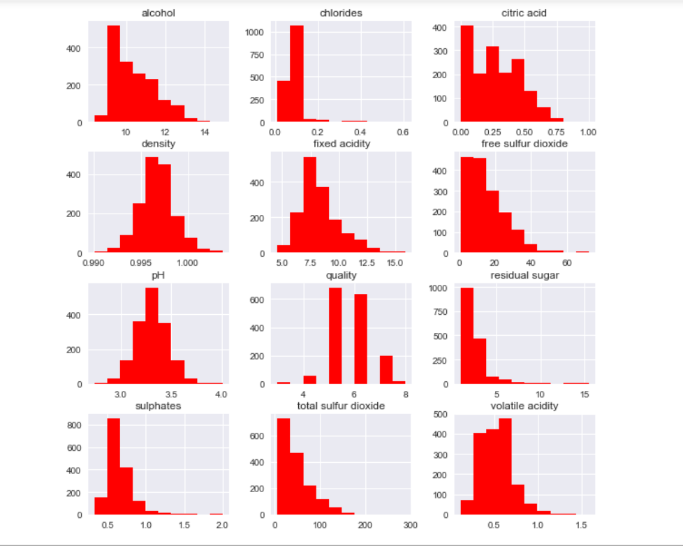
只有质量是离散型变量,主要集中在5和6中,下面分析下变量的相关性:
colormap = plt.cm.viridis
plt.figure(figsize=(12,12))
plt.title('Correlation of Features', y=1.05, size=15)
sns.heatmap(data.astype(float).corr(),linewidths=0.1,vmax=1.0, square=True,
            linecolor='white', annot=True)
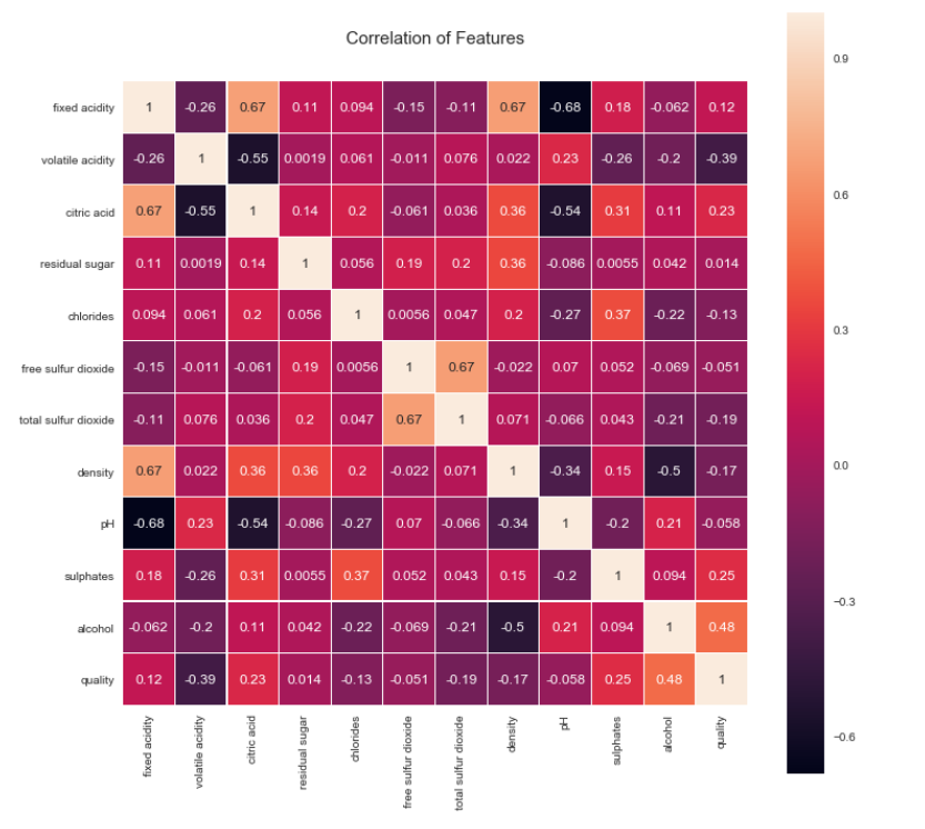
观察:
酒精与葡萄酒质量的相关性最高,其次是各种酸度、硫酸盐、密度和氯化物。
使用分类器:
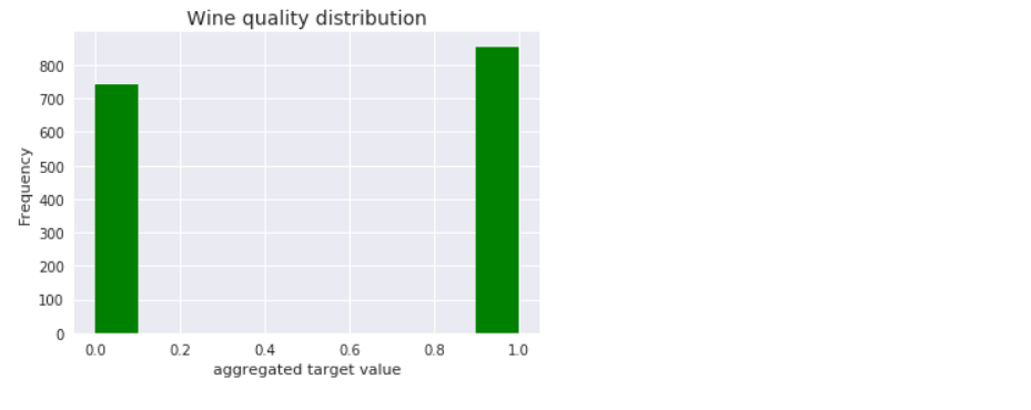
将葡萄酒分成两组;“优质”>5为“好酒”
y = data.quality                  # set 'quality' as target
X = data.drop('quality', axis=1)  # rest are features
print(y.shape, X.shape)           # check correctness

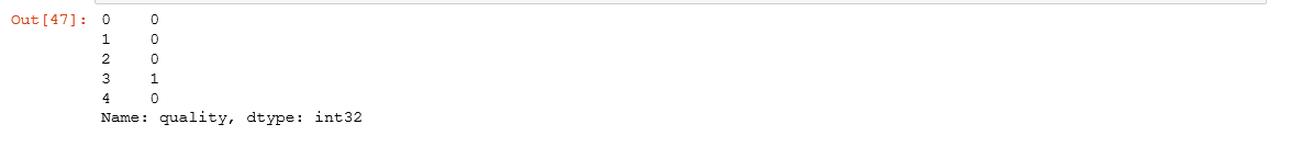
# Create a new y1
y1 = (y > 5).astype(int)
y1.head()
 # plot histogram
ax = y1.plot.hist(color='green')
ax.set_title('Wine quality distribution', fontsize=14)
ax.set_xlabel('aggregated target value')
利用随机森林分类器训练预测模型
from sklearn.model_selection import train_test_split, cross_val_score
from sklearn.ensemble import RandomForestClassifier
from sklearn.metrics import accuracy_score, log_loss
from sklearn.metrics import confusion_matrix
将数据分割为训练和测试数据集
seed = 8 # set seed for reproducibility
X_train, X_test, y_train, y_test = train_test_split(X, y1, test_size=0.2,
                                                    random_state=seed)
print(X_train.shape, X_test.shape, y_train.shape, y_test.shape)

对随机森林分类器进行交叉验证训练和评价
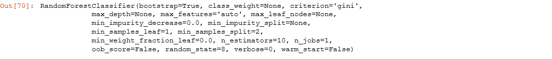
# Instantiate the Random Forest Classifier
RF_clf = RandomForestClassifier(random_state=seed)
RF_clf
# 在训练数据集上计算k-fold交叉验证,并查看平均精度得分
cv_scores = cross_val_score(RF_clf,X_train, y_train, cv=10, scoring='accuracy')
print('The accuracy scores for the iterations are {}'.format(cv_scores))
print('The mean accuracy score is {}'.format(cv_scores.mean()))

执行预测
RF_clf.fit(X_train, y_train)
pred_RF = RF_clf.predict(X_test)
# Print 5 results to see
for i in range(0,5):
    print('Actual wine quality is ', y_test.iloc[i], ' and predicted is ', pred_RF[i])
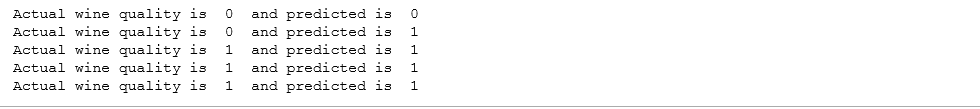
在前五名中,有一个错误。让我们看看指标。
print(accuracy_score(y_test, pred_LR))
print(log_loss(y_test, pred_LR))

print(confusion_matrix(y_test, pred_LR))

总共有81个分类错误。
与Logistic回归分类器相比,随机森林分类器更优。
让我们调优随机森林分类器的超参数
from sklearn.model_selection import GridSearchCV
grid_values = {'n_estimators':[50,100,200],'max_depth':[None,30,15,5],
               'max_features':['auto','sqrt','log2'],'min_samples_leaf':[1,20,50,100]}
grid_RF = GridSearchCV(RF_clf,param_grid=grid_values,scoring='accuracy')
grid_RF.fit(X_train, y_train)
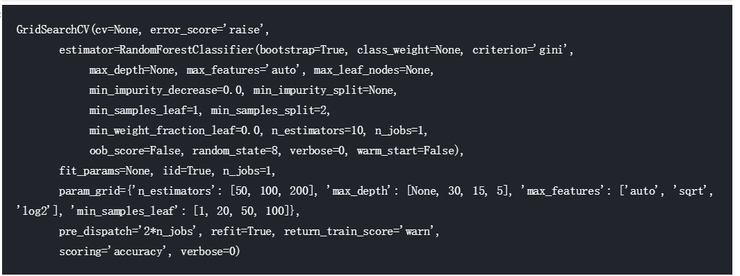
grid_RF.best_params_
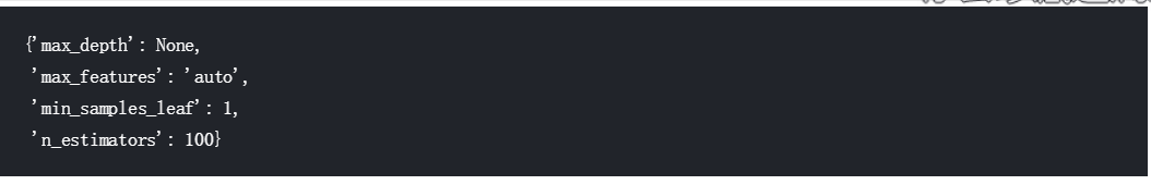
除了估计数之外,其他推荐值是默认值。
RF_clf = RandomForestClassifier(n_estimators=100,random_state=seed)
RF_clf.fit(X_train,y_train)
pred_RF = RF_clf.predict(X_test)
print(accuracy_score(y_test,pred_RF))
print(log_loss(y_test,pred_RF))

print(confusion_matrix(y_test,pred_RF))
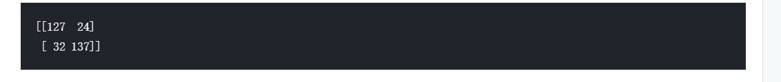
通过超参数调谐,射频分类器的准确度已提高到82.5%,日志损失值也相应降低。分类错误的数量也减少到56个。
将随机森林分类器作为基本推荐器,将红酒分为“推荐”(6级以上)或“不推荐”(5级以下),预测准确率为82.5%似乎是合理的。