To date, the highest accuracy object detector is a two-stage process based on the promotion of R-CNN wherein the classifier is applied to a sparse set of candidate positions. By contrast, the possible target locations for regular, intensive single-stage sampling probe is likely faster and easier, but still far behind the accuracy of the two-stage detector. In this article, we study why this is so. We found that, during training before extreme high-density probe encountered after class imbalance is the main reason. We propose to solve this kind of imbalance by reshaping standard cross-entropy loss, so that it can reduce the loss of the good examples of classification. Our new Focal loss losses concentrated in the example of the difficulties of training a group of sparse, and to prevent a large number of negative samples easily overwhelm the detector detected during training. In order to evaluate the effectiveness of loss, we designed a simple and trained high-density probe, we call RetinaNet. Our results show that when using Focal loss training, RetinaNet can reach the speed of previous single-phase detector, while exceeding all existing most advanced precision two-stage detector. Code is: https: //github.com/facebookresearch/Detectron.
The most advanced target detector is based on a two-stage, proposal-driven mechanism. As R-CNN frame [11] are promoted as the first phase generating a sparse set of position candidates, the second stage uses a convolutional neural network for each candidate position as a foreground or background class category. Through a series of improvements [10,28,20,14], the two phases in the frame can always challenging COCO highest accuracy in the reference [21].
Although the two detectors have been successful, a natural question is: a simple single-stage detector can achieve the same accuracy of a detector used in conventional object location, size and aspect ratio, intensive sampling? . Recent studies on single level detector, such as YOLO [26,27] and SSD [22,9], showing promising results, compared with the most advanced two-stage process, to produce 10-40% Accurate faster detector.
This paper further promote research in this area: the first time we propose a single-stage target detector, which can be matched to the latest COCO AP more complex two-stage detector, such as the characteristics of pyramid network (FPN) [20 ] or Faster R-CNN [28] the Mask R-CNN [14] variant. To achieve this result, we identified the main obstacles imbalance during training is hampered single-stage detector to achieve the most advanced precision, and a new loss function to eliminate this obstacle.
Class in the class imbalance detector R-CNN solved by a two-stage cascade and sampling inspiration. proposal stage (e.g. Selective Search [35], EdgeBoxes [ 39], DeepMask [24, 25], RPN [28]) the number of candidates for the position quickly reduced to a small number (e.g. 1-2k), filter out large part of the background samples. In the second classification phase, heuristics sample, such as a fixed front background ratio (1: 3), or excavation difficulty sample (OHEM) [31], is performed to maintain a manageable balance between the foreground and background .
In contrast, a single-stage process a detector must be set larger location candidates, by which the position of the object image is sampled periodically. In practice, this usually corresponds to enumerate about 100k positions, these positions densely covered space location, size and aspect ratio. Although you can use similar sampling heuristics, but their efficiency is very low, because the training process is still dominated by the background samples easy classification. Such inefficiency is a classical problem in the object detection, the sample is usually tap [37,8,31] and other techniques to guide bootstrapping [33,29] or difficult to solve.
In this paper, we propose a new loss function as a more effective alternative ways to deal with the class imbalance. Cross entropy loss function is a dynamic scaling loss, increased when the confidence of the correct type, the scale factor attenuation is zero, shown in Figure 1:
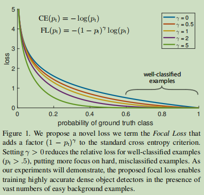
Intuitively, this scaling factor can automatically reduce the training process simple sample of contribution, and quickly model focused on difficult samples . Experimental results show that our proposed Focal loss allows us to accurately train a single level detector, its performance is significantly better than using a sampling or training heuristic methods difficult samples mining, which is a single-stage training detector latest technology . Finally, we note that the exact form of Focal loss is not important, we also show other examples of Keyihuode similar results.
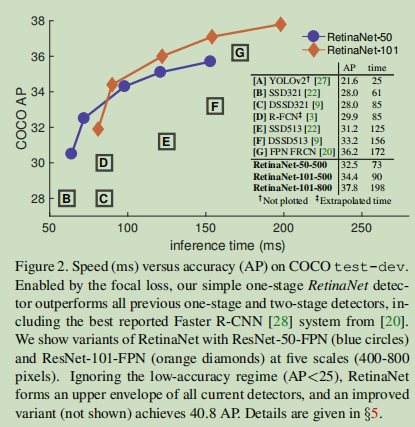
In order to demonstrate the effectiveness of the proposed Focal loss, we designed a simple single-stage target detector, called RetinaNet, its name comes from its densely sampled input image in the target location. It is designed for efficient network features within an anchor boxes pyramid and use. It draws on the latest thinking from [22,6,28,20] of. RetinaNet is efficient and accurate; our best model, based on ResNet-101-FPN trunk, in the case of 5 fps to run under, to achieve the results COCO test-dev AP 39.1, exceeding the previously released from one and two best model results single phase detector, see Figure 2:
Object Detectors Classic : sliding window mode after using a network has a classification method is applied in a dense grid of images, it has a long and rich history. One of the earliest success stories is LeCun and others classics, they will be applied to convolutional neural network handwritten numeral recognition [19, 36]. Viola and Jones [37] using the enhanced object detector for face detection, leading to widespread adoption of such models. Introducing HOG [4] and the integral channel features [5], providing an effective method for the detection of pedestrians. DPMs [8] will help expand intensive probe into the more general subject categories and get many years of top results on PASCAL [7]. Although the sliding window method is a classic computer vision to detect the most important paradigm, but with the depth study [18] of recovery, following the introduction of two detectors soon began to dominate object detection.
Detectors Stage-TWO : Modern Paradigm main object detection is based on two-stage process. Working as selective search [35] of the pioneer, the first stage generating a sparse set of recommended candidates, it should contain all the objects, while filtering out most of the negative sample position, the second phase will suggest as a foreground class / background class. R-CNN [11] The second phase of the upgrade to a convolution classifier network, was a great improvement in the accuracy, ushered in the modern era of target detection. Over the years, R-CNN in speed [15, 10] and on the use of learning objects recommendations [6,24,28] aspects have been improved. Recommended area network (the RPN) of the second stage classifier integrated into a single recommendation generated convolutional network is formed Faster RCNN frame [28]. This framework proposes many extensions, such as [20,31,32,16,14].
Detectors-Stage One : OverFeat [30] is the first network based on the depth of the single-stage object detector. Recently, SSD [22,9] and YOLO [26,27] renewed interest in single-stage process. These detectors have adjusted the speed, but its accuracy behind the two-stage method in. The SSD AP decreased by 10-20%, while focusing on more extreme YOLO speed / accuracy trade-off. See Figure 2. Recent work has shown that as long as the resolution and number of proposals to reduce the input image, the two detectors can work quickly, however, even when a large budget calculation [17], the single-stage method in accuracy still lagging behind. In contrast, the purpose of this work was to understand run at similar or faster, the detector is capable of single-stage match or exceed the precision with which the two detectors.
Design and intensive probe before our RetinaNet detectors have many similarities, especially RPN [28] introduced the "anchors" concept and SSD [22] and [20] use the feature FPN pyramid. We emphasize that our simple detector has been able to achieve the best results, not because of innovations in network design, but because of our new losses.
Imbalance class : either classic single-stage method of detecting an object, such as a boosted detector [37,5] and DPMs [8], or newer methods, such as the SSD [22], in the training process are facing large class unbalanced. The evaluation of each image detectors 10 . 4 -10 . 5 candidate locations, but only a few positions contain objects. This imbalance leads to two questions:
(1) low efficiency of training, most of the places prone to negative samples, no useful learning signal; (2) On the whole, easy to judge negative samples (ie, a large number of background samples) will overwhelm training, leading to the degradation model. A common solution is to perform some form of difficulty sample excavation [33,37,8,31,22], sampling / sample revaluation scheme sampling difficulties during training or a more complex [2]. Instead, we show Focal loss we propose to deal with the kind of natural imbalances faced by single-stage detector, and allow us to conduct effective training on all of the examples, without the need for sampling, did not appear simple judgment negative samples will subvert losses and the calculated gradient.
Estimation, the Robust : Robust people loss function (e.g. Huber loss [13]) is very interested in the function to reduce the weight by reducing the contribution of outliers weight loss of the sample (Sample difficult) having a large error. In contrast, our loss is not the focus of treatment of outliers, but the weight class than to address the imbalance by reducing the rights inliers (simple sample), so that even if a large number of inliers, their contribution to the total loss is small . In other words, Focal loss played with the robustness of the loss the opposite effect: it will focus on the training examples sparse set of difficulties .

Wherein y∈ {± 1} specifies whether the true class (class 1 is represented as a real, non-real -1 represents the class), p ∈ [0,1] is the estimated probability model y = label Class 1 . For ease of marking, we define P T :
FIG CE loss blue (top) curve shown in FIG. 1. A notable properties of this loss is even very easy to classify examples ( i.e., P T is far greater than 0.5 ) will have no small loss. When a large number of simple examples are summed, the value of these small losses may overwhelm a small class (that is not easy to classify the class).
This loss is a simple extension of CE, we will test it as a baseline focal loss of our proposed .
As shown in our experiments, a large number of classes of imbalance in the course of intensive training in the probe encountered offset by cross entropy loss. Easy classification negative samples (i.e., background class) make up the majority of the losses, and led gradient . Although α importance of balancing the positive / negative example, but it is not easy to distinguish / sample difficult. Instead, we recommend reshaping function to reduce weight loss simple weight of the sample, which will focus on training hard negative samples.
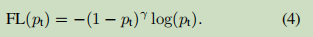
More formally, we propose to add a regulator (. 1 - P T ) gamma] cross-entropy loss, with an adjustable focusing parameters γ≥0. We will define focal loss as:
focal loss γ is set to γ∈ [0, 5] visualize the result of several different weight values shown in Fig. We note that the two focal loss characteristics: (1) When an example is misclassified, and P T value is small ( Description This is a difficult samples ), modulation and focal loss factor is close to 1 is not affected. When p T when → 1, the modulation factor close to 0, the loss for the classification of good samples ( i.e., positive samples tended p 1, p negative samples tends to zero, so that a good simple classification sample p T tends 1 ) to weight loss is declining ( because you want more attention in difficult samples. that is those in the middle of the sample, either positive or negative easily, like this better trained network ). (2) focusing parameter γ smooth adjustment rate decrease simply sample weights. When γ = 0, FL corresponds to CE, when gamma] increases, the Modulation factor also increases (we found that when we set γ = 2 experiments best).
Intuitively, the modulation factor reduces the loss contribution from simple samples, and extends the range of a low-loss sample obtained. For example, γ = 2, an example is classified as P T = 0.9 is reduced 100-fold when compared to the loss of the CE, P T as compared to the 1000-fold loss is reduced when ≈0.968. This in turn increases the importance of correct misclassified examples (for P T ≤0.5 and γ = 2, that loss is scaled up four times, so that this loss is much larger than the loss of easy classification) .
In practice, we use a variant of α-balanced focal loss:
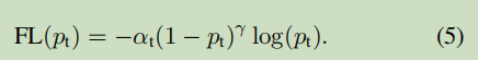
Use of this form of our experiments, no loss of accuracy because it Comparative α-balanced in the form of slightly increased a little. Finally, we note that the connection for the operation of the computing sigmoid loss of p implemented loss layer obtained greater numerical stability.
Although our main results, we use the focal loss defined above, but its precise form is not important. In the appendix, we consider the focal loss of other examples, and prove them equally effective.
By default, the binary classification model is initialized to equal probability output , or 1 to y = -1. In this initialization, in the case of class imbalance, frequent class can lead the overall losses, resulting in instability of early training. To solve this problem, we introduced the concept of "a priori" at the start of training time to represent a rare class (foreground) p-value estimated by the model. We π represents the a priori and it is provided, so that the model used to estimate p-values of rare class is low, for example 0.01. We note that this is a change in the model initialization (see §4.1), rather than the loss of function of the change. We found that in the case of severe class imbalance, which can improve the stability of cross-training and focal loss of entropy.
Two-stage detector is usually trained to use the cross-entropy loss without the use of α-balancing or loss of our proposal. Instead, they are two mechanisms to solve the unbalanced classes: (1) two-stage cascade, and (2) minibatch biased sampling. The first stage is an object proposal cascade mechanism [35,24,28], it will be an almost unlimited number of possible reduction of the target position set to 1000 or 2000. Importantly, the selected proposals is not random, but may be related to the real target corresponding to the position, which eliminates the vast majority of the negative samples easy to judge. In the second stage of training, biased sampling commonly used to construct comprising positive and negative sample ratio of 1: 3 in small quantities. This ratio is like an implicit α-balancing factor achieved by sampling. Our proposed focal loss designed to detect in a single-stage system directly addresses these mechanisms through the loss of function.
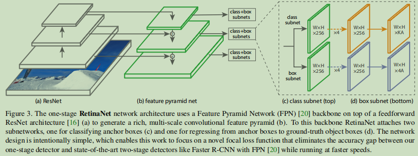
RetinaNet is a single, unified network consists of a backbone network and the sub-network consisting of two specific tasks. Main features responsible for calculating the convolution of the entire input image on the map, a custom convolutional network. A first sub-network backbone convolving output object class; a second sub-network performing convolution bounding box regression. The two subnet has a simple design, we have raised this design, see Figure 3 for a single-stage intensive testing:
Although the details of these components has many possible choices, but most precise design parameter values displayed in the experiment is not particularly sensitive.
Next, we will introduce the various components of RetinaNet.
Pyramid features network backbone : We use features from [20] Pyramid Network (FPN) as a backbone network support. Briefly, the FPN by top-down path and the transverse connection extends the standard convolutional network so that the network can effectively build rich multiscale pyramid features from a single input image resolution, in FIG. 3 (a) - (b) shown in FIG. Each layer of the pyramid can be used to detect objects at different scales. FPN is improved full convolution network (FCN) [23] multiscale predicted from its RPN [28] and DeepMask-style proposals [24] of the improvements, as well as two phase detectors Fast R-CNN [10] or Mask R-CNN [14] the improvement can be seen.
Follow [20], our architecture ResNet [16] on the construction of FPN. We constructed from a P . 3 to P . 7 pyramid, where l denotes the pyramid level ( P l layer 2 has a lower than the input l times the resolution ). In [20], all the pyramid levels have C = 256 channels. Pyramid details usually follow [20], only a few subtle differences. Although many design choices is not important, but we emphasize that it is important to use FPN backbone; Preliminary experiments using only the last layer of the characteristics gained less AP.
Anchors : We use the anchor boxes translation-invariant, similar RPN variants [20] in. In P . 3 to P . 7 pyramid level, anchors 32 are the area of 2 to 512 2 . In [20], in each pyramid level, we use the ratio of the aspect ratio of an anchors three, i.e., {1: 2,1: 1,2: 1}. Ratio [20] more dense coverage scales, we add a size of each layer in the original aspect ratio of three anchors set {2 0 , 2 1/3 , 2 2/3 } times. This improves the AP in our setup. A total of nine each anchor, which cover the network of the input image pixels within the range of 32-813.
Each of the anchors has a length of one-hot vector classification target value K, where K is the number of the target class, and a length of 4 bounding box setpoint vector regression. We use the assignment rules from RPN [28], but for many types of modifications were detected, using the adjusted threshold. Specifically, the use of anchors, and a threshold of 0.5 or more and ratio of the cross (IOU) the anchors will be described as a true target object block; IOU if they are in the range [0, 0.4], then the anchors described background. Since up each assigned to a real object anchors box, we will label the corresponding entry of the vector having a length of K is set to 1, while all other entries set to zero. If a anchors is not allocated ( i.e., not the object frame is not the background ), which shows the results of the anchors IoU between [0.4, 0.5], it is ignored during training. Frame offset between the target return is calculated for each object allocated thereto anchor block, if not allocated, is omitted.
Subnet Classification : Probability A two anchors and K target classes appear in each spatial position in the sub-classification to predict. The subnet is connected to each FPN level of a small FCN network; this parameter subnet shared at all levels of the pyramid. Its design is very simple. FIG obtaining input features a C-channel with a given level of the pyramid, the application subnet four layers of 3 × 3 convolution, each of the layers using C filters, use after each activation function ReLU filter and a convolution with K * a layer of a filter of 3 × 3. Finally, Sigmoid activation function is added into the binary prediction output for each spatial location of the K * A, shown in Figure 3 (c). We used in most experiments c = 256 and A = 9.
And RPN [28] compared to our deeper sub-object classification, only 3 × 3 convs, is not shared with the subnet box regression parameter (to be described later). We find these more advanced design decisions is more important than the specific value exceeds the parameter.
Regression Subnet Box : sub-parallel to the object classification, we will another small FCN network attached to each level of the pyramid, so that each anchor box will return an offset to the real object nearby box (if any). The same block classification and regression subnet subnet design, in addition to the output of the spatial location of each subnet a linear output. 4A, see FIG. 3 (d). A two anchors for each spatial position, the four outputs relative offset between the predicted block and the real anchor (we use the standard frame parameters R-CNN [11]). We note that the recent work different, we use a class unknown bounding box regression, which uses fewer parameters, we find it equally effective. Subnet object classification and regression subnet although sharing the same frame structure, but with different parameters.
4.1. Inference and Training
Corollary: RetinaNet the FCN form a single, a ResNet-FPN from the trunk, a frame and a sub classification regression subnets, see Fig. Thus, a forward inference only involves propagation network image. In order to increase the speed, we only decode the highest prediction score before 1k FPN for each level, and the detector set at 0.05 confidence level. The highest predicted merge all levels, and a non-maximum suppression threshold value of 0.5 to generate a final detection result.
Loss Focal : We used focal loss described in this article as the loss of output sub-classification. §5 we will show, we have found that when γ = 2 when the effect is better in practice, when γ∈ [0.5,5] Robust RetinaNet opposite effect. We emphasize in training RetinaNet, it will be applied to all Focal loss of about 100k more anchors each sample image. This is usually a heuristic sampling (the RPN) or excavation difficulty sample (OHEM, SSD) method of selecting a set of anchor points (e.g., 256) is formed for each small quantities compared. The total focal loss of the image is calculated for all focal loss of about 100k and two anchors, anchors standardized by the number assigned to a real frame. We use the number of anchors allocated to normalize, rather than all of the anchors, because the vast majority of the anchors are likely to be negative, and received the loss of value in the focal loss is negligible. Finally, we should pay attention to the value α, the weighting assigned to the class of rare, there are a range of stable, but simultaneously it is necessary to select a value (Table 1 a and 1 b) these two parameters with γ:
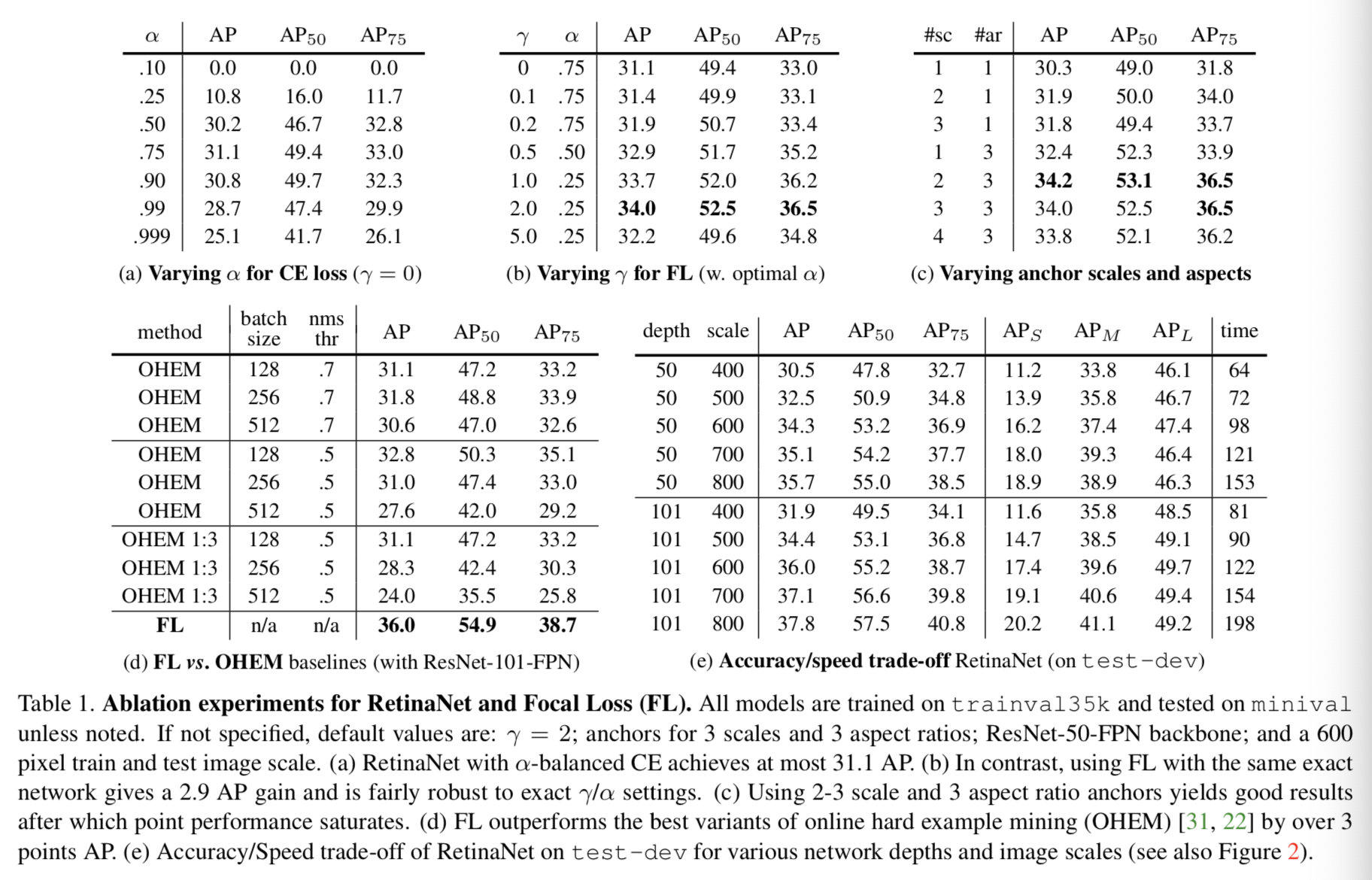
When increased gamma], [alpha] should be generally slightly reduced (γ = 2, α = 0.25 best results).
Initialization : We conducted experiments with ResNet-50-FPN and backbones ResNet-101-FPN [20]. Pre-training base ResNet-50 and ResNet-101 models on ImageNet1k; we use the model [16] published. FPN is initialized to be added to the new layer [20]. RetinaNet conv new subnet all layers except the last layer are initialized to b = 0 and the deviation Gaussian weights using σ = 0.01. Finally, classification of the subnet conv layer, we set the deviation is initialized to b = -log ((1-π ) / π), the [pi] specifies the start of each anchor training should be marked as confidence about the foreground [pi] . In all experiments, we use π =. 01, although the results for the exact value is robust. As explained in §3.3, this initialization can prevent a lot of background anchors have a greater loss of value of the instability in the first iteration of the training.
Optimization : (the SGD) RetinaNet by stochastic gradient descent training methods. We use synchronous SGD on 8 GPU, each minibatch a total of 16 pictures (each GPU 2 photos). Unless otherwise stated, all models have received 90k iterations of training, initial learning rate is 0.01, then divide in the 60k 10, and then divided by 10 in the 80k iterations. Unless otherwise stated, we use horizontal image flip as the only form of data enhancement. 0.0001 weight attenuation value and momentum values 0.9. Training losses by focal loss and return value in block [10] of the standard smoothing L . 1 loss sum. Model training time table 1e 10 to 35 hours.
5. Experiments
Omission
6. Conclusion
In this work, we determine the class imbalance is to prevent a single-stage object detector outside the main obstacle to the best performance of the two-stage method. To solve this problem, we propose a focal loss, it will apply to cross-modulation terms entropy loss, in order to concentrate on learning difficulties negative samples. Our approach is simple and efficient. We prove its effectiveness by designing a full convolution of single-phase detector, and reported a large number of experiments, the results show that it reaches the most advanced precision and speed. Codes are visible https://github.com/facebookresearch/Detectron [ 12 is ]
focal loss visible code for Class-Balanced Loss Based on Effective Number of Samples - 2 - Learning Code