python machine learning - the use of scikit-learn training Perceptron Model

This one we will begin to use scikit-learn API to implement the model and training, this package greatly facilitated our learning process, which includes the implementation of common algorithms, and highly optimized, and contains data preprocessing, tune many ways to participate and model evaluation.

We look at an example've seen before, but this time we use sklearn to train a perceptron models, data sets or Iris, which use two-dimensional features, using sample data 150 samples of all three categories

%matplotlib inline
import numpy as np
from sklearn import datasets

iris = datasets.load_iris()
X = iris.data[:, [2, 3]]
y = iris.target

np.unique(y)

array([0, 1, 2])

In order to assess the predictive power of the model trained on the new data, we will be here Iris data set into training and test sets, here we come to the data set is divided into two parts by calling trian_test_split method, which accounted for 30% of the test set, training set 70%

from sklearn.model_selection import train_test_split
X_train, X_test, y_train, y_test = train_test_split(X, y, test_size=0.3, random_state=0)

We then zoom in features, call here StandardScaler to normalize characteristics:

from sklearn.preprocessing import StandardScaler
sc = StandardScaler()
sc.fit(X_train)
X_train_std = sc.transform(X_train)
X_test_std = sc.transform(X_test)

Sc fit the new object using the method to calculate the mean and standard deviation of the sample data set characteristics in each dimension, and then call a method of transform data sets are normalized, as used herein, we treated the same standardized parameter training and test sets. Then we train a perceptual model

from sklearn.linear_model import Perceptron

ppn = Perceptron(max_iter=40, eta0=0.1, random_state=0)

ppn.fit(X_train_std, y_train)

Perceptron(alpha=0.0001, class_weight=None, early_stopping=False, eta0=0.1,
           fit_intercept=True, max_iter=40, n_iter_no_change=5, n_jobs=None,
           penalty=None, random_state=0, shuffle=True, tol=0.001,
           validation_fraction=0.1, verbose=0, warm_start=False)

y_pred = ppn.predict(X_test_std)

print('Misclassified samples: %d' % (y_test != y_pred).sum())

Misclassified samples: 5

As can be seen on a five test samples are misclassified points, so the error rate is 0.11 classification, the classification accuracy was 1-0.11 = 0.89, we can directly calculate the classification accuracy rate:

from sklearn.metrics import accuracy_score

print('Accuracy: %.2f' % accuracy_score(y_test, y_pred))

Accuracy: 0.89

Finally, we draw the boundary region, where we will make some changes plot_decision_regions function, so that we can distinguish between the training and test sets of samples

from matplotlib.colors import ListedColormap
import matplotlib.pyplot as plt

def plot_decision_regions(X, y, classifier, test_idx=None, resolution=0.02):
    # setup marker generator and color map 
    markers = ('s', 'x', 'o', '^', 'v')
    colors = ('red', 'blue', 'lightgreen', 'gray', 'cyan')
    cmap = ListedColormap(colors[:len(np.unique(y))])
    
    # plot the decision surface
    x1_min, x1_max = X[:, 0].min() - 1, X[:, 0].max() + 1
    x2_min, x2_max = X[:, 1].min() - 1, X[:, 1].max() + 1
    xx1, xx2 = np.meshgrid(np.arange(x1_min, x1_max, resolution),
                          np.arange(x2_min, x2_max, resolution))
    Z = classifier.predict(np.array([xx1.ravel(), xx2.ravel()]).T)
    Z = Z.reshape(xx1.shape)
    plt.contourf(xx1, xx2, Z, slpha=0.4, cmap=cmap)
    plt.xlim(xx1.min(), xx1.max())
    plt.ylim(xx2.min(), xx2.max())
    
    # plot all samples
    X_test, y_test = X[test_idx, :], y[test_idx]
    for idx, cl in enumerate(np.unique(y)):
        plt.scatter(x=X[y == cl, 0], y=X[y == cl, 1], alpha=0.8,
                   c=cmap(idx), marker=markers[idx], label=cl)
    
    # highlight test samples
    if test_idx:
        X_test, y_test = X[test_idx, :], y[test_idx]
        plt.scatter(X_test[:, 0], X_test[:, 1], c='',alpha=1.0,
                   linewidth=1, marker='o', s=55, label='test set')

X_combined_std = np.vstack((X_train_std, X_test_std))

y_combined = np.hstack((y_train, y_test))

plot_decision_regions(X=X_combined_std, y=y_combined, classifier=ppn,
                     test_idx=range(105, 150))
plt.xlabel('petal length [standardized]')
plt.ylabel('petal width [standardized]')
plt.legend(loc='upper left')
plt.show()

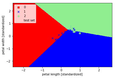
As can be seen in three categories and classified not perfect, this is not linearly separable spent three types of data due.