Linear regression with one variable - Cost function

Abstract: This article is Andrew Ng (Andrew Ng) teacher "machine learning" course, the second chapter "Univariate linear regression" in 7 hours "cost function" of video captions. It was literally in the learning process video recorded for future reference use. Now for everyone to share. If wrong, welcome criticism, to express my sincere thanks! At the same time we want to learn can help.

In this video (article), we'll define something called the cost function. This will let us figure out how to fit the best possible straight line to our data.

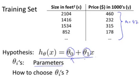
In linear regression we have a training set like that shown here. Remember our notation M was the number of training examples, so maybe M=47. And the form of hypothesis, which we use to make prediction, is this linear function. To introduce a little bit more terminology, this $\theta _{0}$ and $\theta _{1}$ , these $\theta _{i}s$ are what I call the parameters of the model. What we are going to do in this video (article) is talk about how to go about choosing these two parameter values, $\theta _{0}$ and $\theta _{1}$ .

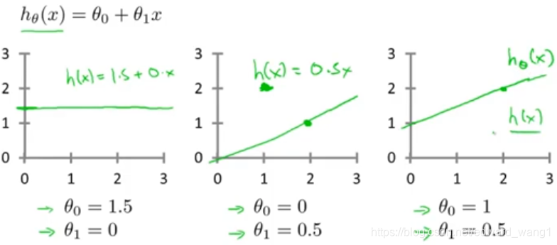
With different choices of parameters $\theta _{0}$ and $\theta _{1}$ we get different hypotheses, different hypothesis functions. I know some of you will probably be already familiar with what I'm going to do on this slide, but just to review here are a few examples. If $\theta _{0}=1.5$ and $\theta _{1}=0$ , then the hypothesis function will look like this. Right, because your hypothesis function will be $h_{\theta }(x)=1.5$ , this is flat at 1.5. If $\theta _{0}=0$ and $\theta _{1}=0.5$ , then the hypothesis will look like this. And this should pass through this point (2,1), says you now have $h_{\theta }(x)=0.5x$ which looks like that. And if $\theta _{0}=1$ and $\theta _{1}=0.5$ , then we end up with the hypothesis that looks like this. Let's see, it should pass through the $(2,2)$ point like so. And this is my new $h_{\theta }(x)$ . All right, well you remember that this is $h_{\theta }(x)$ but as a shorthand, sometimes I just write this as $h(x)$ .

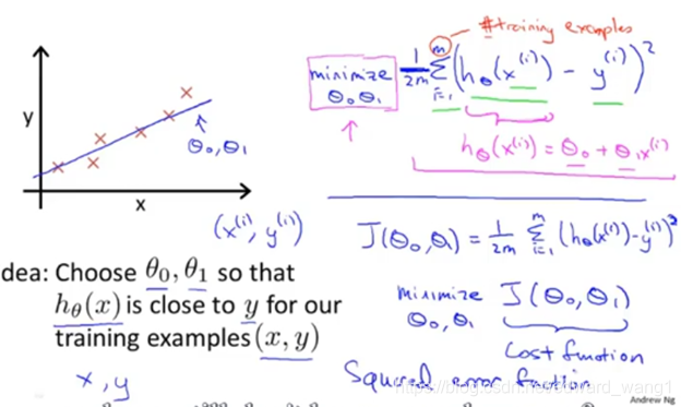
In linear regression we have a training set like maybe the one I've plotted here. What we want to do is come up with values for the parameters $\theta _{0}$ and $\theta _{1}$ . So that the straight line we get out of this corresponds to a straight line that somehow fits the data well. Like maybe the line over there. So how do we come up with values $\theta _{0}$ , $\theta _{1}$ that corresponds to a good fit to the data? The idea is we're going to choose our parameters $\theta _{0}$ and $\theta _{1}$ so that $h_{\theta }(x)$ , meaning the value we predict on input x, that is at least close to the values y for the examples in our training set. So, in our training set we're given a number of examples where we know x decides the house and we know the actual price of what it's sold for. So, let's try to choose values for the parameters so that at least in the training set, given the x's in the training set, we make reasonably accurate predictions for the y values. Let's formalize this. So linear regression, what we're going to do is that I'm going to want to solve a minimization problem. So, I'm going to write minimize over $\theta _{0}$ , $\theta _{1}$ . And, I want this to be small, right, I want the difference between $h_{\theta }(x)$ and y to be small. And one thing I might do is try to minimize the square difference between the output of the hypothesis and the actual price of the house. Okay? So, let's fill in some details. Remember that I was using the notation $(x^{(i)},y^{(i)})$ to represent the $i ^ {th}$ training example. So, what I want really is to sum over my training set. Sum from i to M of the square difference between the prediction of my hypothesis when it is input the size of the house number i, minus the actual price that house number i was sold for and I want to minimize the sum of my training set sum from i equals 1 through M of the difference of this squared error, square difference between the predicted price of the house and the price that was actually sold for. And just remind you of your notation M here was the size of my training set, right, so the M there is my number of training examples, right? That hash sign is the abbreviation for "number" of training examples. Okay? And to make the math a little bit easier, I'm going to actually look at, you know, $1/m$ times that. So, we're going to try to minimize my average error, which we're going to minimize $1 / 2m$ . Putting the 2, the constant one half, in front it just makes some of the math a little easier. So, minimizing one half of something, right, should give you the same values of the parameters $\theta _{0}$ , $\theta _{1}$ as minimizing that function. And just make sure this equation is clear, right? This expression in here, $h_{\theta }(x)$ , this is our usual, right? That's equal to $\theta _{0} + \theta _{1}x^{(i)}$ . And, this notation, minimize over $\theta _{0}$ and $\theta _{1}$ , this means find me the values of theta zero and theta one that causes this expression to be minimized. And this expression depends on $\theta _{0}$ and $\theta _{1}$ . Okay? So just to recap, we're posing this problem as find me the values of $\theta _{0}$ and $\theta _{1}$ so that the average already one over two M times the sum of square errors between my predictions on the training set minus the actual values of the houses on the training set is minimized. So, this is going to be my overall objective function for linear regression. And just to, you know rewrite this out a little bit more cleanly, what I'm going to do by convention is we usually define a cost function. Which is going to be exactly this. That formula that I have up here. And what I want to do is minimize over $\theta _{0}$ and $\theta _{1}$ my function $J(\theta _{0}, \theta _{1})$ . Just write this out, this is my cost function. So, this cost function is also called the squared error function or sometimes called the square error cost function and it turns out that why do we take the square of the errors? It turns out the squared error cost function is reasonable choice and will work well for most problems, for most regression problems. There are other cost functions that will work pretty well, but the squared error cost function is probably the most common used one for regression problems. Later in this class we'll also talk about alternative cost functions as well, but this choice that we just had should be a pretty reasonable thing to try for most linear regression problems. Okay, so, that's the cost function. So far we've just seen a mathematical definition of, you know, the cost function and in case this function $J(\theta _{0}, \theta _{1})$ seems a little bit abstract and you still don't have a good sense of what it's doing, in the next couple of videos (articles) we're actually going to go a little bit deeper into what the cost function J is doing and try to give you better intuition about what it's computing and why we want to use it.

<end>

Linear regression with one variable - Cost function

Guess you like